Jun 4, 2018 - We propose a learned compact feature descriptor tailored for point clouds ..... formance to the results of selected feature descriptors evaluated.
ISPRS Annals of the Photogrammetry, Remote Sensing and Spatial Information Sciences, Volume IV-2, 2018 ISPRS TC II Mid-term Symposium “Towards Photogrammetry 2020”, 4–7 June 2018, Riva del Garda, Italy
LEARNED COMPACT LOCAL FEATURE DESCRIPTOR FOR TLS-BASED GEODETIC MONITORING OF NATURAL OUTDOOR SCENES Zan Gojcic, Caifa Zhou, Andreas Wieser Institute of Geodesy and Photogrammetry, ETH Z¨urich, Zurich, Switzerland (zan.gojcic, caifa.zhou, andreas.wieser)@geod.baug.ethz.ch Commission II, WG II/3 KEY WORDS: Compact feature descriptor, terrestrial laser scanning (TLS), geomonitoring, neural networks, feature-based methods
ABSTRACT: The advantages of terrestrial laser scanning (TLS) for geodetic monitoring of man-made and natural objects are not yet fully exploited. Herein we address one of the open challenges by proposing feature-based methods for identification of corresponding points in point clouds of two or more epochs. We propose a learned compact feature descriptor tailored for point clouds of natural outdoor scenes obtained using TLS. We evaluate our method both on a benchmark data set and on a specially acquired outdoor dataset resembling a simplified monitoring scenario where we successfully estimate 3D displacement vectors of a rock that has been displaced between the scans. We show that the proposed descriptor has the capacity to generalize to unseen data and achieves state-of-the-art performance while being time efficient at the matching step due the low dimension.
1. INTRODUCTION Point clouds have become a standard for dense, digital representation of 3D sceneries. However, beyond visualization and simple distance measurements, raw point clouds are of limited use and mostly serve as a basis for further processing (Hackel et al., 2016). Methods based on feature-extraction and matching nowadays represent the state-of-the-art for processing steps such as coarse registration (Yang et al., 2016), 3D object recognition (Wang et al., 2017), 3D shape retrieval (Bai et al., 2016) and semantic classification (Hackel et al., 2016). Local feature descriptors are key elements of the feature-based methods. They represent information about the local geometry and radiometry around individual points and have to be descriptive enough such that the nearest neighbors in feature space refer to points with similar local geometry and radiometry.
objects like rocks may translate and rotate but not deform over time. The approach presented herein will later allow deriving 3D displacement vectors, which can be tested statistically for significance and can be used for a more rigorous deformation analysis properly taking into account rigid body motion and actual deformation. The paper is structured as follows: We propose a 3D feature descriptor tailored for point clouds of natural outdoor scenes in Section 3 and address the high time complexity of the matching step due to the high-dimensional feature vectors (Gawel et al., 2017) in Section 4. In Section 5, we show the results of the proposed approach on a selected benchmark dataset and indicate the applicability of the method for geodetic monitoring by estimating the 3D displacement of individual rocks in a scanned scenery. 2. RELATED WORK
Point clouds derived from terrestrial laser scanning (TLS) are increasingly used to detect and quantify displacements and deformation of man-made and natural structures in geodetic monitoring. In comparison to the traditional geodetic methods based on precise measurements to individual, carefully selected and marked points, areal-based techniques for data acquisition, like TLS, allow detecting changes at non-expected locations (Wunderlich et al., 2016). However, multiple challenges remain unresolved in deformation analysis based on TLS (Holst and Kuhlmann, 2016), in particular parameterization of deformations and quantification of error probabilities like false alarm rate or probability of missed detection. These challenges are solved for individual, repeatedly measured points but not for point clouds. We address this challenge herein by proposing feature-based methods for the identification of corresponding points in point clouds of two or more epochs. This paves the way to the identification of stable areas, deformed areas and areas or objects which transformed rigidly between the measurement epochs. A typical application case would be the monitoring of a landslide where parts of the repeatedly scanned scene may be stable over time while others change due to the flow of earth and debris, and larger
2.1
Local feature descriptors
Over the last decades, hand-crafted feature descriptors were developed and proposed for specific tasks especially in 3D computer-vision and robotics. For example, Johnson and Hebert (1999) proposed the descriptor referred to as spin images, where the neighborhood of each query point is represented by a 2D histogram of cylindrical coordinates w.r.t. the normal vector at the point. Rusu et al. (2008) proposed a feature descriptor for automatic coarse registration denoted as point feature histogram (PFH). It is a histogram of the angular variations and distances between points and their normal vectors in the neighborhood of the respective query point, calculated using Darboux frames between pairs of points. Due to the high computational complexity Rusu et al. (2009) later proposed a more efficient version of PFH referred to as fast point feature histogram (FPFH). Frome et al. (2004) proposed a 3D generalization of the 2D shape context descriptor denoted as 3DSC. They use a local point density feature (as we do herein) computed in a subdivided local spherical neighborhood. However, the spherical grid is not unique and an individual descriptor needs to be computed for each subdivision in
This contribution has been peer-reviewed. The double-blind peer-review was conducted on the basis of the full paper. https://doi.org/10.5194/isprs-annals-IV-2-113-2018 | © Authors 2018. CC BY 4.0 License.
113
ISPRS Annals of the Photogrammetry, Remote Sensing and Spatial Information Sciences, Volume IV-2, 2018 ISPRS TC II Mid-term Symposium “Towards Photogrammetry 2020”, 4–7 June 2018, Riva del Garda, Italy
azimuth. Tombari et al. (2010b) later showed that the descriptiveness can be improved by establishing a unique and unambiguous local reference frame (LRF) at the query point for subdividing its neighborhood into spatial bins. Tombari et al. (2010a) significantly improved the performance of 3DSC just by establishing such an LRF. Similarly, a LRF was also used in Tombari et al. (2010b) for computing the signature of histograms of orientations (SHOT) descriptor, which uses the normal vector deviations (also used herein). SHOT has been identified as still one of the best performing feature descriptors in a recent extensive evaluation by Guo et al. (2016). Inspired by the recent success of (convolutional) neural networks (NNs) in 2D computer vision, researchers have also proposed learned feature descriptors. However, such descriptors either require a volumetric representation which can be very computationaly expensive e.g., Zeng et al. (2017), or cannot capture local finegrained structures see e.g., Qi et al. (2017). Furthermore, they are not intrinsically invariant to rotations and try to overcome this by augmenting the data with random rotations (usually only around the up-axis). We will present an approach herein where a handcrafted high-dimensional feature descriptor is used as an input to a NN. This approach is similar to the ones proposed by Fang et al. (2015) and Khoury et al. (2017). With growing size of point clouds, time and memory efficiency of the feature descriptors have become crucial, especially for larger scenes. Particularly the matching step can be very time consuming (Gawel et al., 2017). Researchers tackled this issue by dimensionality reduction using e.g. principal component analysis, e.g. (Johnson and Hebert, 1999). This reduces the computational burden but comes at the cost of matching performance. On a related note, several binary feature descriptors that can exploit a very fast computation of the Hamming distance were proposed, e.g. the local feature descriptor proposed by (Dong et al., 2017). Transferring the feature-based approaches to applications based on point clouds representing natural scenes with quasi-random structures and collected under changing environmental conditions represents a special challenge (Wagner et al., 2016). 2.2
Geomonitoring using TLS point clouds
Ohlmann-Lauber and Sch¨afer (2011) categorized deformation models for monitoring based on point clouds into five categories: point-based, point cloud-based, surface-based, geometry-based and parameter-based models. Natural outdoor scenes typically have surfaces which cannot be described analytically. So, deformation analysis in geomonitoring is predominantly based on point cloud- and surface-based models (Neuner et al., 2016) assuming that the point clouds from different epochs are registered. For example, the well-established Cloud to Cloud (C2C) method yields the distance between each point of the data point cloud and its nearest neighbor in the reference point cloud. However, the field of 3D displacement vectors thus obtained does not (necessarily) connect corresponding points, and is therefore very difficult to interpret. Lague et al. (2013) proposed a Multiscale Model to Model Cloud Comparison (M3C2) and showed its applicability on the survey of a complex 3D river canyon. Using M3C2 the distance between points from two different epochs is measured along the direction of the normal vector of a plane fitted to the respective point’s vicinity. Additionally, a parametric confidence interval denoted as level of detection (LOD) can be obtained from the point clouds
and enables statistical significance testing of the computed deformations. However, this method is only sensitive to deformation or displacement in a predefined direction, namely perpendicularly to the respective surface. Rigid body motion is not easily detected from such an analysis, and deformation components along the surface are not indicated. Indeed, geomonitoring beyond quantification of subsidence requires correspondence between points to be established irrespective of the spatial direction of the changes. This requires establishing correspondence based on features extracted from the data. Wagner et al. (2017) proposed a fusion of laser scanning and image data using standard image feature descriptors (SIFT and BRISK) to match the corresponding points and derive the 3D displacement vectors from the associated point clouds. Herein we present an approach using directly the geometry within the point cloud for establishing correspondence. 3. HIGH-DIMENSIONAL LOCAL GEOMETRIC FEATURE DESCRIPTOR A local feature descriptor has to encapsulate the predominant information of a point’s neighborhood in order to distinguish this point from other points in a point cloud (Guo et al., 2016). To enable matching of corresponding points in two point clouds when they are not represented in the same coordinate system (e.g. nonregistered scans of the same scene) or when the corresponding object has been rigidly displaced, the extracted feature representation should be invariant under rigid transformation. The state-of-the-art feature descriptors (Tombari et al., 2010a; Guo et al., 2014; Salti et al., 2014) which achieve the best performance in the assessment by Guo et al. (2016), ensure a translation and rotation invariant representation of the point’s neighborhood by expressing the local features in a unique, repeatable LRF. The repeatability refers to the property that the estimated LRF is object-oriented and should thus be equal for the corresponding point in two or more point clouds of the same scenery when estimated independently for each of them. Petrelli and Di Stefano (2011) showed that the probability of successful matching deteriorates rapidly with decreasing repeatability of the LRF. The datasets typical for geomonitoring are especially challenging for the estimation of repeatable LRFs because of the high noise level and typically ragged surfaces. The approach proposed herein takes this into account by expressing the features with respect to a local reference axis (LRA) instead of a complete LRF. We use a robustly estimated normal vector to define the LRA because this is an intrinsically well-defined direction that can be estimated with high repeatability (Petrelli and Di Stefano, 2011). We then combine two types of features that showed good performance in the recent evaluation by Guo et al. (2016): the local point density feature proposed by Frome et al. (2004) and adopted by Tombari et al. (2010a), and the normal vector deviations feature proposed by Tombari et al. (2010b). A detailed explanation of both LRA establishment and local feature extraction is given in the remainder of this section. 3.1
Local reference axis
Given a point p in the point cloud P we select its local spherical support S⊂P such that S = {pi : kpi − pk2 ≤ rLRA }, where rLRA denotes the radius of the neighborhood used for the estimation of the LRA. The eigenvector corresponding to the smallest ˆ S then corresponds eigenvalue of the sample covariance matrix Σ
This contribution has been peer-reviewed. The double-blind peer-review was conducted on the basis of the full paper. https://doi.org/10.5194/isprs-annals-IV-2-113-2018 | © Authors 2018. CC BY 4.0 License.
114
ISPRS Annals of the Photogrammetry, Remote Sensing and Spatial Information Sciences, Volume IV-2, 2018 ISPRS TC II Mid-term Symposium “Towards Photogrammetry 2020”, 4–7 June 2018, Riva del Garda, Italy
3.2
Figure 1. Segmentation of the local spherical support of the query point p into spatial bins along the radial and elevation direction. Point pi is assigned to the spatial bin Fjk (depicted with grey background color). to the total least squares estimate of the surface normal. However, the total least squares estimation is very sensitive to outliers. Therefore, we first select a robust subset Q ⊂ S and estimate the surface normal using this robust subset. Specifically, we filter the outliers using the highly robust deterministic minimum covariance determinant (det-MCD) estimator of the mean-value and covariance matrix proposed by Hubert et al. (2012). Given a dataset with a observations in b dimensions, the objective of the det-MCD is to find h observations1 whose covariance matrix has the smallest determinant while b(a + b + 1)/2c ≤ h ≤ a. Using only these h observations the robust estimates of the mean ˆ MCD,S of S are computed. ˆ MCD,S and the covariance matrix Σ µ We then compute the Mahalanobis distance based on these estimates as q ˆ −1 ˆ MCD,S )T Σ ˆ MCD,S ) (1) dM (pi , S) = (pi − µ MCD,S (pi − µ and select Q such that Q = {qi : qi ∈ S ∧ dM (qi , S) ≤ λ}, where we set the cut-off value to λ = 3.06 which corresponds to q
χ20.975,3 , i.e. the cut-off value proposed by the authors in Hubert et al. (2012). Nurunnabi et al. (2014) empirically showed that this is a suitable threshold for the surface normal estimation in unordered point clouds although we cannot assume the points ˆ MCD,S . The LRA is then parto be normally distributed around µ ˆ (a) at point p obtained as allel to the estimated normal vector n the eigenvector corresponding to the smallest eigenvalue of the ˆ Q . To choose the sign of the robust sample covariance matrix Σ LRA we adopt the sign disambiguation method from Bro et al. ˆ such that the (2008) which yields the sign of the normal vector n −→ is positive. This inner product of the majority of the vectors − pp i is achieved by ( 1, if hˆ n(a) , (pi − p)i ≥ 0 1S (pi ) = 0, otherwise �P � (2) ( ˆ (a) , if n 1 (p ) ≥ 0.5|S| S i pi ∈S ˆ= n −ˆ n(a) , otherwise where | · | denotes the cardinality of the set.
1 In Experiments presented in Section 5 we use h = 0.75|S| as proposed by the authors in Hubert et al. (2012) and Nurunnabi et al. (2014).
High-dimensional feature descriptor
A local feature descriptor has to be invariant to translation and rotation of the coordinate system or point cloud while also being descriptive enough to enable successful matching of the corresponding points. Herein, we use two types of features for the high-dimensional description of the local surface geometry each of them evaluated for spatial bins about the query point. For the binning we first determine a local spherical support F of the query point p. F is chosen like S in Section 3.1 but using the feature radius rf instead of rLRA .2 We then segment the local neighborhood defined by rf into spatial bins by dividing the sphere into nr sections along the radial dimension and into nα sections in terms of elevation (see Figure 1), where elevation is defined as the deflection angle from the LRA. The radial bins are spaced logarithmically by adopting the method from Frome et al. (2004) for calculating the lower and upper limits of the bins: ( 0, if j = 0 rj = (3) rf j exp(ln rmin + nr ln( rmin )), otherwise Logarithmic spacing assigns larger weights to the points in the vicinity of the query point by reducing the size of the bins close to it, while rmin is the size of the first bin and is used to avoid overly excessive binning at or next to the query point. The elevation direction is subdivided into nα equally sized bins such that the lower and upper limits of the bins are given by αk = nkπα , k = 0, . . . , nα . For each of the ns = nα · nr spatial bins we compute two types of features, the local point density and the normal vector deviation. For calculating the local point density we assign each point pi ∈ F to one of the spatial bins Fjk based on its location relative to point p as pi ∈ Fjk ⇔ kpi − pk2 ∈ (rj , rj+1 ] ∧ cos−1 (hˆ n, (pi − p)i) ∈ (αk , αk+1 ]
(4)
We then normalize the number of points in each spatial bin with |F|. For the normal vector deviation we follow Tombari et al. (2010b). In each spatial bin we compute cos θi , where θi denotes ˆ at the query point and the angle between the normal vector n ˆ pi at each point lying within that spatial bin. the normal vector n The cosine is used as a measure of normal vector deviation as it ˆ|n ˆ pi . Within can be easily computed according to cos θi = n each individual spatial bin nn equally spaced normal deviation bins covering the range from −1 to 1 are then defined and the number of deviations within each bin is counted. These numbers are normalized using the respective |Fjk | such that they sum up to 1 within each spatial bin. Finally, for each point of the point cloud all these features are collected into a high-dimensional feature descriptor fhd (pi ) of dimension ns ·(nn +1). In the experiments presented in Section 5, we use nr = nα = nn = 10 such that the feature descriptor is of dimension 1100. 4. FEATURE EMBEDDING INTO A LOWER-DIMENSIONAL SPACE Once the feature vectors are computed, they can be used to determine the corresponding points in two point clouds using some sort of a nearest-neighbour search for purposes like registration or monitoring. This can be very time inefficient. In2 Note,
that rf should be larger than rLRA .
This contribution has been peer-reviewed. The double-blind peer-review was conducted on the basis of the full paper. https://doi.org/10.5194/isprs-annals-IV-2-113-2018 | © Authors 2018. CC BY 4.0 License.
115
ISPRS Annals of the Photogrammetry, Remote Sensing and Spatial Information Sciences, Volume IV-2, 2018 ISPRS TC II Mid-term Symposium “Towards Photogrammetry 2020”, 4–7 June 2018, Riva del Garda, Italy
Figure 2. Siamese network architecture. Local features of an anchor point xi , positive example xpi and negative example xn i are extracted and fed to the fully connected Siamese neural network (yellow squares). The output layer (blue squares) represents the intermediate representation used for feature matching in the online stage. All branches of the network share all the parameters. deed, e.g. the brute-force algorithm query will scale approximately as O(DN 2 ), where D denotes the dimension of the feature vector and N denotes the number of points. Using treebased methods (e.g. kd-tree) this can be reduced to approximately O(DN log(N )) for small D, but still becomes inefficient when D grows large. This is known as the ”curse of dimensionality”, Weber et al. (1998). The curse of dimensionality can be mitigated using approximate nearest neighbor algorithms or dimensionality reduction. We opt for dimensionality reduction using a deep NN that maps the high-dimensional feature vector (c.f. Section 3) into a lower-dimensional feature space. The gain is twofold: • by reducing the dimension of the feature vector, the nearest neighbor search can be performed much faster; • with fine-tuning the non-linear mapping can be optimized for a specific application (e.g. for processing point clouds of natural objects).
4.1
Network architecture
Given a 1100 dimensional feature vector fhd ∈ RD, D = 1100, a multilayer perceptron (MLP) i.e., a NN fθ , is constructed for embedding the high-dimensional feature vector fhd into a lower dimensional feature space. So, fθ (fhd ) ∈ Rd , d � D, where θ denotes the parameters of the NN. This multi-layer NN is designed as a Siamese network (Bromley et al., 1994) consisting of several identical branches (three branches are used herein) which share all the parameters (i.e. the number of nodes, weights and biases, and activation functions of each layer), see Figure 2. Herein we train a Siamese network to learn the similarity of the positive and dissimilarity of the negative pair of examples in a triplet, i.e. |E| E = {(fhd (xi ), fhd (xpi ), fhd (xn i ))}i=1 represents the training set, where fhd (xi ) denotes the high-dimensional feature vector of the i-th anchor point, fhd (xpi ) denotes a chosen positive sample and fhd (xn i ) a negative one. The details of sampling these training triplets are given in Section 4.2. The advantage of using a Siamese network is that the learning process is self-supervised (or unsupervised) which simplifies the application of the proposed approach to geomonitoring by allowing generation of an appropriate training data set from a pair of pre-aligned point clouds with sufficient overlap. In order to optimize the parameters of the NN, we minimize the following contrastive loss function L(θ) us-
ing stochastic gradient descent (SGD) in the framework of backpropagation: L(θ) =
|E| 1 X kfθ (fhd (xpi )) − fθ (fhd (xi ))k2 |E| i=1 kfθ (fhd (xn i )) − fθ (fhd (xi ))k2
(5)
This can be seen as a type of a triplet loss (Khoury et al., 2017), thus training the network to minimize the distance between corresponding feature vectors while at the same time maximizing the distance between dissimilar ones. The architecture of the NN used herein consists of four fully connected (FC) hidden layers, which contain 1024, 512, 512, and 256 nodes respectively, each followed by a rectified linear unit (ReLU) activation function for non-linear mapping to a 32-dimensional feature space (see Figure 2). We use mini-batches and train the mapping fθ using Adam (Kingma and Ba, 2015). The initial weights of the hidden nodes are initialized using Xavier initialization (Glorot and Bengio, 2010). The learning rate is set to 1.5 × 10⁻⁴ . The parameters for the exponential decay of the first and second moment estimates are set to β1 = 0.9 and β2 = 0.999. The network is trained with an early stopper (see Section 4.3). We determine parameters of the NN with the grid search method using the point clouds from the Bologna 3D Retrieval benchmark dataset (see Section 5.2). The NN was implemented in Python using TensorFlow.3 4.2
Sampling of the training triplets
Let P = {Pi }; i = 1, . . . , N be a set of overlapping point clouds of a scene. In this work, we assume that a set T = {Tji }; i, j = 1, . . . , N of transformations for pairwise alignment of the point clouds (indices i and j) is given or can be readily obtained using registration. Consider two specific point clouds Pi and Pj . For each point p ∈ Pi we search the nearest neighbor q ∈ Tij (Pj ) and select this point as a positive example. When training the network it is important to feed the network with hard negatives, i.e. points that are different but similar to the anchor point, in order to ensure good performance and fast convergence (Schroff et al., 2015). Intuitively, hard negative examples lie in the vicinity of the anchor point. Therefore, for each point p ∈ Pi we search for a set U of neighbors in Tij (Pj ) such that U = {ui : 0.5 · rf < kp − ui k2 < 1.5 · rf } where rf 3 https://www.tensorflow.org/
This contribution has been peer-reviewed. The double-blind peer-review was conducted on the basis of the full paper. https://doi.org/10.5194/isprs-annals-IV-2-113-2018 | © Authors 2018. CC BY 4.0 License.
116
ISPRS Annals of the Photogrammetry, Remote Sensing and Spatial Information Sciences, Volume IV-2, 2018 ISPRS TC II Mid-term Symposium “Towards Photogrammetry 2020”, 4–7 June 2018, Riva del Garda, Italy
is as defined in Section 3. The lower limit of 0.5 · rf is selected because we treat all the points that are closer to the anchor point as potentially correct matches. We build the training triplets as follows: we randomly sample 10 hard negatives from U and augment them by randomly sampling 10 points from the rest of the point cloud in order to avoid overfitting to the surrounding of the anchor point. Additionally, we copy the anchor point and the positive example 20 times to fill all the triplets. Thus forming 20 training examples for each point in the point cloud. 4.3
Early stopping regularization
Figure 3. Bunny and Dragon models from the B3R dataset. Red color denotes the front part and blue color the back one as used for separate fine-tuning of the descriptor.
To mitigate the over-fitting problem during training of the NN early stopping is introduced into the training process (Erhan et al., 2010). Therefore, the training of the NN is stopped when the predefined maximum number of epochs is reached or when a different, more specific condition is fulfilled. The condition applied herein is the occurrence of three consecutive drops of the average recall (as defined in Equation 7) of the training epochs. For computing the average recall of an epoch, we average all the recall values (τ = 1) in one epoch computed using one minibatch as the validation set, after training the NN with 50 minibatches.4
The two feature vectors fiR and fiD are considered a match if kfiR −fiD k2 ≤ τ for a given value of τ . Further, the match is kf R −f D k
5. EXPERIMENTS
and recall denotes the number of correct matches versus the number of corresponding features
In this section we apply the proposed low-dimensional feature descriptor and briefly assess the results. First, we test the descriptiveness and robustness on the Bologna 3D retrieval (B3R) benchmark dataset (Tombari et al., 2013) and compare the performance to the results of selected feature descriptors evaluated by Yang et al. (2017)5 . Second, we indicate the applicability of the proposed descriptor for use in geomonitoring by applying it to a scanned scenery with rocks (RB3D dataset). Third, we evaluate the time complexity of the nearest neighbor search in feature space. The parameters used in this evaluation are presented in Table 1. 5.1
Accuracy metric
Given two point clouds, i.e. a reference point cloud PR and a data point cloud PD , we assume that the transformation parameters aligning PD and PR are given. We follow the evaluation procedure used by Yang et al. (2017). We randomly sample a set R of 1000 points from PR and search for a set D of corresponding points from PD aligned to PR , i.e. the respective nearest neighbors. Then we compute the feature vectors as described in Sections 3 and 4. Let fiR denote the feature vector of the i-th point of R, and fiD and fiD0 those of the nearest and the second nearest neighbor (in terms of l2 -norm) in D Dataset
rLRA [mm]
rmin [mm]
rf [mm]
batch size
B3R RB3D
15 40
5 7
25 50
64 64
Table 1. Parameters used for computation of the feature descriptor in the experiments presented herein.
4 While computing the recall during a training epoch, the number of corresponding points equals the batch size, i.e. 64. 5 In Figure 4 we report the results of the SHOT descriptor because the best performing descriptor is not publicly available.
i
i0
2
considered correct if the coordinate distance between the points is less than 10 times the point cloud resolution of the reference cloud, where the point cloud resolution equals the median distance between each point of PR and its nearest neighbor. Otherwise, the match is considered false. We use the precision-recall curve (PRC) as evaluation criterion. The precision denotes the number of correct matches versus the number of all matches precision =
recall =
# of correct matches # of all matches
# of correct matches # of corresponding points
(6)
(7)
The PRC is obtained by varying τ ∈ (0, 1]. Additionally, we provide the Area under the Curve (AUC) value as a scalar indicator of overall performance of the descriptor. A high AUC represents both, heigh precision and heigh recall. 5.2
Bologna 3D retrieval dataset (B3R)
The B3R dataset consist of 18 scenes derived from six 360◦ models which are originally part of the Stanford 3D Scanning Repository. The scenes are rigidly-transformed copies of the models with three levels of added Gaussian noise. Herein, we only use the scenes with 0.1 mesh resolution one sigma standard deviation. Of those, we use the Armadillo, Buddha, Chinese Dragon and Statuette data sets for training, and Bunny and Dragon as test datasets. We perform the split such that the test dataset contains one model with lower resolution and predominantly smooth surfaces (Bunny) and one model with higher resolution and partially ragged surface (Dragon). We train the NN for 11 epochs and then test the learned descriptor on the Bunny and Dragon models. The results, depicted in Figure 4 (left), show that our learned descriptor has the capacity to generalize to unseen data. We can further increase the performance of the descriptor by fine-tuning it to the point density and geometric structures that are specific for an individual model. Therefore, we divide the test models into the front and back parts as denoted in Figure 3 and use one of them for fine-tuning the pre-trained model and the other one for testing. The number of points in the training dataset in relation to the batch size is approximately three times higher for the Dragon model than for the Bunny model. Therefore, we stop the fine-tuning process after three epochs for the former and after one epoch for the latter. The final performance of the learned descriptors is presented in Figure 4 (right). The average AUC using the low-dimensional descriptor proposed herein equals 0.74 for Bunny, 0.85 for Dragon and 0.79 on average for both models from the B3R data set. The best performing descriptor in
This contribution has been peer-reviewed. The double-blind peer-review was conducted on the basis of the full paper. https://doi.org/10.5194/isprs-annals-IV-2-113-2018 | © Authors 2018. CC BY 4.0 License.
117
100
100
90
90
80
80
70
70
Precision [%]
Precision [%]
ISPRS Annals of the Photogrammetry, Remote Sensing and Spatial Information Sciences, Volume IV-2, 2018 ISPRS TC II Mid-term Symposium “Towards Photogrammetry 2020”, 4–7 June 2018, Riva del Garda, Italy
60 50 40 30
60 50 Bunny-front [0.708] Bunny-back [0.773] Dragon-front [0.843] Dragon-back [0.851] SHOT - B3D [0.696]
40 30
Bunny [0.654] Dragon [0.750] SHOT - B3D [0.696]
20 10 0
10
20
30
40
20 10
50
60
70
80
90
100
Recall [%]
0
10
20
30
40
50
60
70
80
90
100
Recall [%]
Figure 4. Results of the learned low-dimensional feature descriptor on the B3R dataset models Bunny and Dragon compared to the results of the SHOT descriptor on all models as reported by Yang et al. (2017). Values in squared brackets denote the AUC. Left: Performance after learning the model for 11 epochs on the training dataset. Right: Performance after fine-tuning the model for 3 epochs (Bunny) and 1 epoch (Dragon), respectively. Bunny-front denotes that the NN was fine-tuned using the Bunny-back and tested on the Bunny-front. Interpretation of the other labels is correspondingly. the comparative study by Yang et al. (2017) achieved an AUC of 0.76 on average for the six models with 0.1 mesh resolution of noise. While this might suggest that our descriptor performs slightly better, it is just a first indication because the values refer to an average performance over six models using a different support size (15 times mesh resolution i.e. approx. 20 mm) than the one used herein. A comprehensive performance assessment is not a primary goal of this publication and is left for future work. 5.3
Simulated monitoring of an outdoor scenery (RB3D)
We demonstrate the applicability of the proposed feature descriptor to TLS-based geomonitoring using point clouds from a real outdoor scenery, denoting the dataset as rigid body 3D (RB3D). Two rocks with a diameter of approximately 0.5 m are located next to seven boulders (diameter up to approximately 3 m), see Figure 5. The scene has been scanned three times using a Faro Focus3D X330 terrestrial laser scanner from a distance of approximately 15 m and using an angular sampling interval of 0.018◦ . This resulted in more than 1.9 M points for each of the three epochs. Between epochs 1 and 2, we moved the scanner by about 1 m; the resulting point clouds represent an unchanged scene in different coordinate systems. Between epochs 2 and 3 one of the two small rocks (displaced rock) was moved by about 1.5 m and rotated by approximately 5◦ around a vertical axis while the scanner and the other rock (stable rock) remained at the same position. In this way we simulate a use case where a landslide would be scanned several times over a certain period of time, some parts of the scene remaining constant during that period and others moving. By moving the scanner between epochs 1 and 2 we attempt
to incorporate some of the nuisances which may affect the point clouds of repeated scans of the unchanged scene. For preparation, the scans were roughly aligned manually and then coregistered using ICP. Points representing vegetation were removed in order to reduce the number of points in each point cloud and restrict the analysis to the part of the pointclouds representing boulders and rocks. We then computed the high dimensional feature descriptor for all three epochs and used points of the stable rock and displaced rock from epochs 1 and 2 for training of the neural network (NN). The performance was evaluated using the point clouds from epochs 2 and 3. As a consequence of displacing and rotating the displaced rock, a lot of nuisances for the feature descriptors are introduced. As the rock is closer to the scanner, the resolution of the point cloud increases and the footprint of the laser beam gets smaller (less smoothing). Additionally, due to the displacement of the rock different parts are occluded and the incidence angle of the laser beam for individual points changes. Nevertheless, more than 1700 points from displaced rock and more than 4800 points from stable rock (approximately 12 % and 20 % of the overlap respectively) were correctly matched at τ = 1. The search space. i.e. the point cloud of epoch 2, contained approximately 0.8M points. Areas that were correctly matched and the consequently derived 3D displacement vectors are presented in Figure 6. Many object have similar surfaces in the scanned scenery. So, many points were erroneously matched. However, the correct matches can be identified using filtering or integration of some prior knowledge. In this particular example, we assumed that individual rocks were rigidly displaced but not deformed. In this case the correct matches referring to the same objects or to objects undergoing the same rigid body motion cor-
Figure 5. Point cloud of the geomonitoring scenery (first epoch). Stable natural environment is indicated by grey color (intensity). Rocks, which where placed in the scenery are displayed in color: stable rock (red), displaced rock (blue = first epoch, green = third epoch).
This contribution has been peer-reviewed. The double-blind peer-review was conducted on the basis of the full paper. https://doi.org/10.5194/isprs-annals-IV-2-113-2018 | © Authors 2018. CC BY 4.0 License.
118
ISPRS Annals of the Photogrammetry, Remote Sensing and Spatial Information Sciences, Volume IV-2, 2018 ISPRS TC II Mid-term Symposium “Towards Photogrammetry 2020”, 4–7 June 2018, Riva del Garda, Italy
Figure 6. Results of the RB3D experiment for displaced rock: second epoch (orange), third epoch (blue). Green color denotes the points that were correctly matched. For clarity we only show 20 derived 3D displacement vectors. respond to a single set of transformation parameters. RANSAC was used in our example to identify these matches and the corresponding transformation of the displaced rock. To obtain correct matches we set the inlier threshold in RANSAC to 10 times the point cloud resolution. 5.4
Time complexity of the descriptor
We analyze the time needed to perform the nearest neighbor search on the RB3D dataset using the high-dimensional feature descriptor (see Section 3) and its low-dimensional embedding (see Section 4. We only analyze the time complexity of the dimensionality reduction using NN and the matching step, because the computation of the high-dimensional feature vector was not optimized (single-thread implementation in Python). Specifically, we use the Scikit-learn machine learning library6 implementation of the nearest neighbor search in Python on a standalone desktop PC with Intel Xeon E5-1650 CPU v4 (hexa-core, 3.60 GHz) and 32 GB of RAM for this analysis. We use the k-d tree implementation of the nearest neighbor search for both descriptors and additionally a brute-force search for the high dimensional feature descriptor. Points are sampled randomly for this analysis. The results are presented in Figure 7. For the low-dimensional feature descriptor they contain the joint time needed for embedding the feature vector and performing the nearest neighbor search; for all implementations they cover samples sizes up to the respective maximum which the computer could handle. The low-dimensional feature descriptor clearly outperforms the high-dimensional one regarding time complexity of 103
Time [ms]
6. CONCLUSION We have proposed a low-dimensional feature descriptor tailored for point clouds of natural outdoor scenes. Considering typical characteristics of the natural objects, we express local features (normal vector deviation and local point density) with respect to a robustly estimated LRA. Furthermore, we address the high time complexity of the matching step by implementing a NN based dimensionality reduction. In the numerical examples used for evaluation, reduction of the dimension of the feature vector from the initial 1100 to 32 reduced the time needed to search for corresponding points by a factor of up to 1200. We showed that we can achieve a state-of-the-art performance with a feature vector of only 32 dimensions on the B3R dataset. Using a dedicated experiment we indicated the applicability of the feature-based method for geomonitoring correctly estimating the rigid-body displacement of a single rock in a natural outdoor scenery from the displacement of corresponding feature points identified using the proposed descriptor. Future work will include a test of the performance of our approach on real geomonitoring data, and the implementation of a rigorous deformation analysis model capable of differentiating between stable, rigidly transformed and actually deformed parts of a scenery. References Bai, S., Bai, X., Zhou, Z., Zhang, Z. and Jan Latecki, L., 2016. Gift: A real-time and scalable 3d shape search engine. In: Proceedings of the IEEE Conference on Computer Vision and Pattern Recognition, pp. 5023–5032. Bro, R., Acar, E. and Kolda, T. G., 2008. Resolving the sign ambiguity in the singular value decomposition. Journal of Chemometrics 22(2), pp. 135–140.
low-dim (k-d) high-dim (k-d) high-dim (brute)
102
the nearest neighbor search, especially when evaluating larger datasets. For particularly small datasets (less than 1000 points) the brute-force algorithm outperforms the k-d tree implementation due to the overhead time needed to build the tree. Considering the largest dataset for which all the implementations could be computed in this test (50k points), the k-d tree search with the low-dimensional feature vector takes about 0.11 ms per query. It is approximately 35 times faster than the brute force search with the high-dimensional feature vector (3.84 ms). Due to the curse of dimensionality (search space grows approximately exponentially), the k-d tree search with the high-dimensional feature vector (68.13 ms) performs approximately 600 times slower than with the low-dimensional feature vector.
Bromley, J., Guyon, I., LeCun, Y., S¨ackinger, E. and Shah, R., 1994. Signature verification using a” siamese” time delay neural network. In: Advances in Neural Information Processing Systems, pp. 737–744.
101 100
Dong, Z., Yang, B., Liu, Y., Liang, F., Li, B. and Zang, Y., 2017. A novel binary shape context for 3d local surface description. ISPRS Journal of Photogrammetry and Remote Sensing 130(Supplement C), pp. 431 – 452.
−1
10
10−2 2 10
103
106
Erhan, D., Courville, A. and Vincent, P., 2010. Why Does Unsupervised Pre-training Help Deep Learning? Journal of Machine Learning Research 11, pp. 625–660.
Figure 7. Time needed for querying the nearest neighbor of one point in the dataset.
Fang, Y., Xie, J., Dai, G., Wang, M., Zhu, F., Xu, T. and Wong, E., 2015. 3d deep shape descriptor. In: Proceedings of the IEEE Conference on Computer Vision and Pattern Recognition, pp. 2319–2328.
6 http://scikit-learn.org/
104 No. of Points
105
This contribution has been peer-reviewed. The double-blind peer-review was conducted on the basis of the full paper. https://doi.org/10.5194/isprs-annals-IV-2-113-2018 | © Authors 2018. CC BY 4.0 License.
119
ISPRS Annals of the Photogrammetry, Remote Sensing and Spatial Information Sciences, Volume IV-2, 2018 ISPRS TC II Mid-term Symposium “Towards Photogrammetry 2020”, 4–7 June 2018, Riva del Garda, Italy
Frome, A., Huber, D., Kolluri, R., B¨ulow, T. and Malik, J., 2004. Recognizing objects in range data using regional point descriptors. In: ECCV, Springer, pp. 224–237.
Qi, C. R., Su, H., Mo, K. and Guibas, L. J., 2017. Pointnet: Deep learning on point sets for 3d classification and segmentation. In: CVPR, pp. 77–85.
Gawel, A., Dub, R., Surmann, H., Nieto, J., Siegwart, R. and Cadena, C., 2017. 3d registration of aerial and ground robots for disaster response: An evaluation of features, descriptors, and transformation estimation. In: 2017 IEEE International Symposium on Safety, Security and Rescue Robotics (SSRR), pp. 27–34.
Rusu, R. B., Blodow, N. and Beetz, M., 2009. Fast point feature histograms (fpfh) for 3d registration. In: Robotics and Automation, 2009. ICRA’09. IEEE International Conference on, IEEE, pp. 3212–3217.
Glorot, X. and Bengio, Y., 2010. Understanding the difficulty of training deep feedforward neural networks. In: Proceedings of the Thirteenth International Conference on Artificial Intelligence and Statistics, pp. 249–256. Guo, Y., Bennamoun, M., Sohel, F., Lu, M., Wan, J. and Kwok, N. M., 2016. A comprehensive performance evaluation of 3d local feature descriptors. International Journal of Computer Vision 116(1), pp. 66–89. Guo, Y., Sohel, F., Bennamoun, M., Lu, M. and Wan, J., 2014. Rotational projection statistics for 3D local surface description and object recognition. International Journal of Computer Vision 105, pp. 63–86. Hackel, T., Wegner, J. D. and Schindler, K., 2016. Fast semantic segmentation of 3d point clouds with strongly varying density. In: ISPRS Annals of Photogrammetry, Remote Sensing & Spatial Information Sciences, Vol. 3number 3, pp. 177–184. Holst, C. and Kuhlmann, H., 2016. Challenges and present fields of action at laser scanner based deformation analyses. Journal of applied geodesy 10(1), pp. 17–25. Hubert, M., Rousseeuw, P. and Verdonck, T., 2012. A deterministic algorithm for robust location and scatter. Journal of Computational and Graphical Statistics 21, pp. 618–637. Johnson, A. E. and Hebert, M., 1999. Using spin images for efficient object recognition in cluttered 3d scenes. IEEE Transactions on pattern analysis and machine intelligence 21(5), pp. 433–449. Khoury, M., Zhou, Q.-Y. and Koltun, V., 2017. Learning compact geometric features. In: Proceedings of the IEEE Conference on Computer Vision and Pattern Recognition, pp. 153–161. Kingma, D. P. and Ba, J. L., 2015. Adam: a Method for Stochastic Optimization. In: International Conference on Learning Representations 2015, pp. 1–15. Lague, D., Brodu, N. and Leroux, J., 2013. Accurate 3d comparison of complex topography with terrestrial laser scanner: Application to the rangitikei canyon (n-z). ISPRS Journal of Photogrammetry and Remote Sensing 82, pp. 10 – 26. Neuner, H., Holst, C. and Kuhlmann, H., 2016. Overview on current modelling strategies of point clouds for deformation analysis. AVN Allgemeine Vermessungs-Nachrichten 123, pp. 328– 339. Nurunnabi, A., Belton, D. and West, G., 2014. Robust statistical approaches for local planar surface fitting in 3d laser scanning data. ISPRS Journal of Photogrammetry and Remote Sensing 96(Supplement C), pp. 106 – 122. Ohlmann-Lauber, J. and Sch¨afer, T., 2011. Ans¨atze zur ableitung von deformationen aus tls-daten. In: 106. DVW Seminal Terrestrisches Laserscanning-TLS 2011 mit TLS-Challenge, Hotel Esperanto Fulda, pp. 147 – 157. Petrelli, A. and Di Stefano, L., 2011. On the repeatability of the local reference frame for partial shape matching. In: Proceedings of the IEEE International Conference on Computer Vision, pp. 2244–2251.
Rusu, R. B., Blodow, N., Marton, Z. C. and Beetz, M., 2008. Aligning point cloud views using persistent feature histograms. In: 2008 IEEE/RSJ International Conference on Intelligent Robots and Systems, pp. 3384–3391. Salti, S., Tombari, F. and Di Stefano, L., 2014. SHOT: Unique signatures of histograms for surface and texture description. Computer Vision and Image Understanding 125, pp. 251–264. Schroff, F., Kalenichenko, D. and Philbin, J., 2015. Facenet: A unified embedding for face recognition and clustering. In: Proceedings of the IEEE Conference on Computer Vision and Pattern Recognition, pp. 815–823. Tombari, F., Salti, S. and Di Stefano, L., 2010a. Unique shape context for 3d data description. In: Proceedings of the ACM Workshop on 3D Object Retrieval, 3DOR ’10, ACM, New York, NY, USA, pp. 57–62. Tombari, F., Salti, S. and Di Stefano, L., 2010b. Unique signatures of histograms for local surface description. Lecture Notes in Computer Science (including subseries Lecture Notes in Artificial Intelligence and Lecture Notes in Bioinformatics) 6313 LNCS(PART 3), pp. 356–369. Tombari, F., Salti, S. and Di Stefano, L., 2013. Performance evaluation of 3d keypoint detectors. International Journal of Computer Vision 102(1-3), pp. 198–220. Wagner, A., Wiedemann, W. and Wunderlich, T., 2017. Fusion of laser scan and image data for deformation monitoring concept and perspective. In: 7th International Conference on Engineering Surveying (INGEO), pp. 157–164. Wagner, A., Wiedemann, W., Wasmeier, P. and Wunderlich, T., 2016. Improved concepts of using natural targets for geomonitoring. In: Joint International Symposium on Deformation Monitoring (JISDM), Vol. 3. Wang, J., Lindenbergh, R. and Menenti, M., 2017. Sigvox–a 3d feature matching algorithm for automatic street object recognition in mobile laser scanning point clouds. ISPRS Journal of Photogrammetry and Remote Sensing 128, pp. 111–129. Weber, R., Schek, H.-J. and Blott, S., 1998. A quantitative analysis and performance study for similarity-search methods in high-dimensional spaces. In: International Conference on Very Large Data Bases, pp. 194–205. Wunderlich, T., Niemeier, W., Wujanz, D., Holst, C., Neitzel, F. and Kuhlmann, H., 2016. Areal deformation analysis from tls point clouds the challenge. AVN Allgemeine VermessungsNachrichten 123, pp. 340–351. Yang, B., Dong, Z., Liang, F. and Liu, Y., 2016. Automatic registration of large-scale urban scene point clouds based on semantic feature points. ISPRS Journal of Photogrammetry and Remote Sensing 113, pp. 43 – 58. Yang, J., Zhang, Q. and Cao, Z., 2017. The effect of spatial information characterization on 3D local feature descriptors: A quantitative evaluation. Pattern Recognition 66, pp. 375– 391. Zeng, A., Song, S., Nießner, M., Fisher, M., Xiao, J. and Funkhouser, T. A., 2017. 3dmatch: Learning local geometric descriptors from rgb-d reconstructions. In: 2017 IEEE Conference on Computer Vision and Pattern Recognition (CVPR), pp. 199–208.
This contribution has been peer-reviewed. The double-blind peer-review was conducted on the basis of the full paper. https://doi.org/10.5194/isprs-annals-IV-2-113-2018 | © Authors 2018. CC BY 4.0 License.
120