Learning Adversary-Resistant Deep Neural

Learning Adversary-Resistant Deep Neural Networks Qinglong Wang1,2 , Wenbo Guo1,3 , Kaixuan Zhang1 , Alexander G. Ororbia II1 , Xinyu Xing1 , C. Lee Giles1 , and Xue Liu2 1

arXiv:1612.01401v1 [cs.LG] 5 Dec 2016

Pennsylvania State University 2 McGill University 3 Shanghai Jiao Tong University Abstract—Deep neural networks (DNNs) have proven to be quite effective in a vast array of machine learning tasks, with recent examples in cyber security and autonomous vehicles. Despite the superior performance of DNNs in these applications, it has been recently shown that these models are susceptible to a particular type of attack that exploits a fundamental flaw in their design. This attack consists of generating particular synthetic examples referred to as adversarial samples. These samples are constructed by slightly manipulating real datapoints in order to “fool” the original DNN model, forcing it to mis-classify previously correctly classified samples with high confidence. Addressing this flaw in the model is essential if DNNs are to be used in critical applications such as those in cyber security. Previous work has provided various defense mechanisms by either augmenting the training set or enhancing model complexity. However, after a thorough analysis, we discover that DNNs protected by these defense mechanisms are still susceptible to adversarial samples, indicating that there are no theoretical guarantees of resistance provided by these mechanisms. To the best of our knowledge, we are the first to investigate this issue shared across previous research work and to propose a unifying framework for protecting DNN models by integrating a data transformation module with the DNN. More importantly, we provide a theoretical guarantee for protection under our proposed framework. We evaluate our method and several other existing solutions on both MNIST, CIFAR-10, and a malware dataset, to demonstrate the generality of our proposed method and its potential for handling cyber security applications. The results show that our framework provides better resistance compared to state-of-art solutions while experiencing negligible degradation in accuracy.

I. I NTRODUCTION Beyond highly publicized victories in automatic gameplaying as in Go [33], there have been many successful applications of deep neural networks (DNN) in image and speech recognition. Recent explorations and applications include those in medical imaging [2], [38] and self-driving cars [10], [14]. In the domain of cybersecurity, security companies have demonstrated that deep learning could offer a far better way to classify all types of malware [8], [30], [39]. However, though powerful, deep neural architectures, as well as all other machine learning methods, break down in the face of adversarial learning [3], [17], where such systems can be easily deceived by non-obvious and potentially dangerous The first and second author contributed equally.

manipulations [24], [35]. To be more specific, prior work [11] has shown that an attacker could use the same algorithm used to train these models, back-propagation of errors, and a surrogate dataset to construct an auxiliary model that can accurately approximate the target DNN model. Compared to the original model that usually returns categorical classification results (e.g., benign or malicious software), such an auxiliary model could provide the attacker with useful details about a DNN’s weaknesses (e.g., a continuous classification score for a malware sample). As such, the attacker can use the auxiliary model to examine class/feature importance and identify the features that have significant impact on the target’s classification ability. Armed with this knowledge of feature importance, the attacker can more easily craft an adversarial sample, or synthetic example generated by slightly perturbing a real example such that the original DNN model believe it belongs to the wrong class with high confidence. Recently, this flaw inherent in machine learning has been widely exploited to fool DNNs trained for image recognition (e.g., [24]) and malware classification (e.g., [12]). In the past, research in hardening deep learning relies on the assumption of security through obscurity. As we will discuss in this paper, this assumption typically does not hold in many real world scenarios. In addition, the techniques proposed (e.g., [11], [13], [25], [34]) can only be empirically validated and cannot provide any theoretical guarantees. This is particularly disconcerting when they are applied in security critical applications such as malware detection. In this work, we relax assumptions made in past research, and propose a framework to facilitate the design of adversaryresistant DNNs. More specifically, we assemble a data transformation module in front of a standard DNN. With this data transformation module, the original input data samples are projected into a new representation before it is passed through the successive DNN. This can be used as a defense since data transformation can potentially conceal the space of adversarial manipulations to a carefully designed hyperspace, making feature/class examination difficult. Following our proposed framework, we implemented a DNN which takes a non-parametric dimensionality reduction method to transform input data to a new representation. We theoretically prove the DNN developed in this manner can be

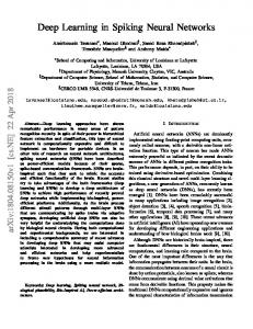
A. Deep Neural Networks A typical DNN architecture, graphically depicted in Fig. 1, consists of multiple successive layers of processing elements, or so-called “neurons”. Each processing layer can be viewed as learning a different, more abstract representation of the original multidimensional input distribution. As a whole, a DNN can be viewed as a highly complex function that is capable of nonlinearly mapping original high-dimensional data points to a lower dimensional space. A DNN contains an input layer, multiple hidden layers, and an output layer. The input layer

f(x) ...

II. BACKGROUND In this section, we first briefly introduce the well-established DNN model. Then we describe the adversarial learning problem. Specificaly, we summarize existing ways one could “attack” a DN and then generalize these attacks under a unified framework.

x ...

adversary-resistant. In addition, we empirically demonstrate this adversary-resistant DNN exhibits high classification accuracy. Last, we compare our adversary-resistant DNN with existing defense mechanisms in the context of image recognition and malware classification. The results show that the proposed adversary-resistant DNN provides strong resistance to adversarial samples while the other defense mechanisms only demonstrate limited effectiveness. To be best of our knowledge, this work is the first to provide DNNs with theoretically guaranteed resistance to adversarial samples. In addition, our adversary-resistant DNN can maintain desirable classification performance while having minimal modification to existing DNN. Last but not least, our proposed framework are generally applicable to deep learning applications covering a broad research interest. In summary, this work makes the following contributions. • We propose a general framework to facilitate the development of adversary resistant DNNs. More specifically, we stack a data transformation module in front a standard DNN which conceals the space of adversarial manipulations in a carefully designed hyperspace. • Using the framework, we develop an adversary-resistant DNN, and theoretically prove its resistance to adversarial manipulation. • We empirically evaluate the classification performance of our adversary-resistant DNN in the context of image recognition and malware classification, and compare it with existing defense mechanisms. The rest of this paper is organized as follows. Section II introduces the background of DNNs and the generation of adversarial samples. Section III discusses a strong assumption of the threat model adopted in previous work and then refines this threat model by relaxing this assumption. Section IV presents our proposed general framework and Section V develops an adversary-resistant DNN under our framework. In Section VI, we evaluate our developed DNN on three datasets. Section VII summarizes existing defense mechanisms. Finally, we conclude this work in Section VIII.

L(f(x), y ) Loss Function

Input Layer

Hidden Layers

Softmax Layer

Figure 1: Neural network architecture: here we depict a simple neural network with three hidden layers, with interconnections between all neurons in each layer, but no intralayer connections. This architecture is referred to as a feedforward neural network [4].

takes in each data sample in the form of a multidimensional vector. Starting from the input, computing the activations of each subsequent layer simply requires, at minimum, a matrix multiplication (where a weight/parameter vector, with length equal to the number of hidden units in the target layer, is assigned to each unit of the layer below) usually followed by summation with a bias vector. This process roughly models the process of a layer of neurons integrating the information received from the layer below (i.e., computing a pre-activation) before applying an elementwise activation function1 . This integrate-then-fire process is repeated subsequently for each layer until the last layer is reached. The last layer, or output, is generally interpreted as the model’s predictions for some given input data, and is often designed to compute a parameterized posterior distribution using the softmax function (also known as multi-class regression or maximum entropy). This bottomup propagation of information is also referred to as feedforward inference [15]. During the learning phase of the model, the DNN’s predictions are evaluated by comparing them with known target labels associated with the training samples (also known as the“ground truth”). Specifically, both predictions and labels are taken as the input to a selected cost function, such as cross-entropy. The DNN’s parameters are then optimized with respect to this cost function using the method of steepest gradient descent, minimizing prediction errors on the training set. Parameter gradients are calculated using back-propagation of errors [32]. Since the gradients of the weights represent their influence on the final cost, there have been multiple algorithms developed for finding optimal weights more accurately and efficiently [23]. More formally, given a training set (X, Y ): 1 There are many types of activations to choose from, including the hyperbolic tangent, the logistic sigmoid, or the linear rectified function, etc. [4]

{(x1 , y1 ), (xn , yn ), . . . , (xn , yn )}, where xi ∈ Rm is a data sample and yi ∈ Rk is data label, where, if categorical, is typically represented through a 1-of-k encoding. A standard neural network with a softmax output layer can be represented by the following function: f : Rm → Rk x 7→ f (x).

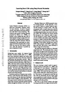
Fast gradient sign

(1)

The cost function for training a DNN as a (k-class) classifier is also defined as follows: L : Rm × Rk → R f (x) × y 7→ L(f (x), y).

(2)

B. Adversarial Sample Problems Even though a well-trained neural network is capable of recognizing some unseen data samples, such a model has been shown to be easily fooled by introducing perturbations to the input that are often indistinguishable to the human eye [35], as shown in Fig.2. These so-called “blind spots”, or adversarial samples, exist because the input space of the DNN is broad [11]. Knowing this, we can uncover specific data samples in the input space that “bypass” DNN models. More specifically, it was shown in [11] that attackers can find the most powerful blind spots using effective optimization procedures. In multi-class classification tasks, such adversarial samples can cause a DNN to classify a data point into a random class other than the correct one (sometimes not even a reasonable alternative). Adversarial samples are generated by computing the derivative of the cost function with respect to the network’s input variables. The gradient of any input sample represents a direction vector in the model’s high-dimensional input space. Along this direction, an small change in this input sample can cause the DNN to generate a completely different prediction result. This particular direction is important since it represents the most effective way one might compromise the optimization of the cost function. Discovering this particular direction is realized by transmitting the error gradients from output layer all the way back to the input layer via back-propagation. The gradient with respect to the input may then be applied to the input sample(s) to craft an adversarial example(s). We now formally present the generation of adversarial samples by first defining the function g for generating any adversarial sample x ˆ: g : R m × Rk → Rm

(3)

x × y 7→ x ˆ, where

x ˆ = arg max L(f (ˆ x), y) x ˆ

(4)

s.t. kˆ x − xkp < ε,

Figure 2: Adversarial samples: we demonstrate adversarial examples generated from MNIST dataset [20] and CIFAR-10 dataset [19]. Images on the left panel are adversarial examples generated by fast gradient sign [11]. For each column in the left panel, we use x, ε and x ˆ to denote original images, generated perturbations and the corresponding adversarial samples. Images on the right panel are generated by solving (4) by L-BFGS and p is set to 2 [21].

Note that g is a one-to-one mapping, meaning that when there exist multiple x ˆ satisfying (4), only one is chosen. It should be noted that the constraint in (4) ensures that the distortion incurred by manipulation must be maintained at a small scale. Otherwise a significant distortion will leave the manipulation to be easily detected.2 Existing attacks [7], [11], [28], [35] consist of different approaches for generating adversarial samples. These approaches, ultimately, can all be described solving following optimization problem, which is a transformation of (4): min c kx − x ˆkp − L(f (ˆ x), y), x ˆ

(6)

where c is some weight or coefficient. Here we refer to this type of attack as an optimal attack, and, for simplicity, denote kx − x ˆkp as the lp distance. Solving (6) is done much like solving for the weight coefficients of a standard DNN. Simply put, an attacker can use back-propagation and either gradient descent [11] or LBFGS [7], [35]. In order to conduct the calculation, one first computes ∂ n L(f (ˆ x), y)/∂ x ˆn and then use it for manipulating legitimate samples x. Note that here n = 1 if we use a first-order optimization method like gradient descent, or n = 2 if we utilize a second-order method such as the Newton–Raphson method [6]. Since gradient descent requires an iterative calculation, it can be computationally expensive when the number of adversarial samples to be generated is large. To mitigate this problem, [11] proposed the fast gradient

and k·kp is p-norm: kvkp =

n X i=1

! p1 |vi |

p

.

(5)

2 However, it was explained in [25], that while easily-detectable, applying greater amounts of distortion still yields an easily-recognizeable image for humans. Given this, the classifier should still be able to correctly classify the sample.

sign method to approximate this iterative calculation where one could use a single step of gradient descent, as follows: x ˆ = x +  · sign(∇L(f (x), y)),

(7)

where  is set to control the scale of the distortions applied. Due to its computational efficiency, the fast gradient sign has been widely used in multiple studies [11], [13], [25]. Optimal attacks can be generalized to fast gradient sign attacks by selecting the l∞ distance. In [35], the authors study an equivalent optimization problem to (6) by setting p = 2. Another type of attack, as described in [28], generates adversarial samples using a greedy approach to solve (6) and sets p = 0. More specifically, adversarial samples are crafted by iteratively perturbing one coordinate of x at a time. A coordinate is picked by determining by its influence on the final cost. C. End-to-end Gradient Flow In order to solve (6), previously introduced attacks must be able to calculate the n-th order 3 derivative of L(f (ˆ x), y) with respect to x ˆ. The calculation of ∂ n L(f (ˆ x), y)/∂ x ˆn requires the existence of an end-to-end gradient flow between the final objective and the input. More formally, given a DNN F 4 with cost function L, for any pair of input sample x and target label y, if ∂ n L(F (x), y)/∂xn can be computed by passing residual error ∂ n L(F (x), y)/∂F (x)n backwards to the input through intermediate layers of a (fully-differentiable) DNN, then we say there exists an end-to-end gradient flow. Existing attacks [7], [11], [27], [35] generate adversarial sample x ˆ by exploiting the existence of an end-to-end gradient flow. As long as the DNN supports end-to-end gradient flow, it will always be susceptible to adversarial perturbation.

refer to the threat model in this case as the black box threat model and adversarial samples generated under it as black box adversarial samples. B. Limitations As introduced in Section I, a relatively large fraction of adversarial examples generated from one trained DNN will be misclassified by the other DNNs trained using the same dataset but with different hyper-parameter settings. Therefore, an adversary can easily generate effective adversarial samples to bypass standard DNN classifiers, by exploiting well known training algorithms and training datasets. More importantly, this information disclosure can also be exploited to attack previously proposed defense mechanisms. To make this issue clearer, we contrast the case of neural network adversarial training algorithms against cryptology. In real world scenarios, any secure encryption algorithm can be freely disclosed to the public without suffering from attacks. The black-box assumption underlying the current threat model does not hold in practice. Indeed, given the publicity and the limited number of existing mechanisms, in practice, it is not difficult for an adversary to enumerate the solutions and design new adversarial samples crafted specifically for attacking the current forms of defense. Note that as previously discussed, access to the training algorithm is sufficient to “break” a DNN–an adversary does not need access to the exact form of the model and its defense mechanism. As will be shown later in Section IV, existing defense mechanisms suffer exactly the same threat for standard DNNs. Since the assumption discussed above is too strong to be of practical use in real world scenarios, we relax this assumption and present a white box threat model in the following sub-section.

III. T HREAT M ODEL In this section, we first describe the threat model that previous research has assumed and then discuss the limitations of this particular threat model. In light of this, we develop a new practical threat model. A. The Black Box Threat Model Existing defense mechanisms [11], [13], [25], [34] are designed to handle the threat directly imposed on standard DNNs (and other differentiable models, including simple linear ones). Specifically, these defenses only focus on defending adversarial samples generated from standard DNNs. While these mechanisms have yielded promising results, the scope of their provided robustness is restricted to standard DNNs and similar differentiable models. This undesired restriction is the result of a strong assumption shared by all of these defenses– the attacker does not know of the adversarial learning algorithm used to “harden” the target DNN. In other words, these mechanisms themselves are assumed (perhaps inadvertently) to be black boxes to adversaries. In consideration of this, we 3 Note

that in this problem, n = 1 or 2. is different from f , f represents a standard DNN, F refers to any neural network architecture, of which the standard DNN is one example of. 4F

C. The White Box Threat Model Under the white box threat model, an adversary is assumed to be able to generate adversarial samples specifically crafted for a target DNN. Furthermore, our proposed white box threat model covers two important cases. One is the extreme case where the exact information about a target DNN is known to the adversary. This corresponds to the first, innermost region in Fig. 3. The other case is that only the training algorithm, the DNN structure, and the dataset(s) used to build the target DNN can be accessed or inferred by adversaries. This corresponds to the second region in Fig. 3. The latter case is more likely as it is similar to the case of generating cross-model adversarial samples from standard DNNs. Nonetheless, we also consider the first case since it represents the most potent threat to DNNs. We refer to adversarial samples generated under the white box threat model as white box adversarial samples 5 . Black box adversarial samples are shown in the third outermost region in Fig. 3. 5 Note that a large fraction of white box adversarial samples are generated under the second case mentioned before. These samples are also fall under the category of cross-model adversarial samples [11].

Feed Forward Transformation

Deep Neural Networks

Input X

Loss Function

...

End-to-end Gradient Flow

Figure 4: Adversary-resistant DNN framework: the proposed framework consists of a data transformation module g(·) and a DNN f (·). In the feed-forward pass, input data is first projected to a certain manifold. Then the transformed data g(X) is used to train a standard DNN classifier. The end-to-end gradient flow (marked by the bold red line) is blocked by the input data transformation module. This module also ensures that recovering original data X from the transformed data g(X) is computationally intractable.

1 : Model-specific adversarial samples 1+2: White box adversrial samples 3: Black box adversarial samples

2 1

2

The first design goal requires that our proposed framework facilitate the development of truly adversary-resistant DNNs. The second design goal requires that any proposed framework preserve the classification (or predictive) accuracy of DNN models when confronted with legitimate samples.

3

B. Framework

Figure 3: Relationship between different sets of adversarial samples: darker colors indicate that the corresponding attack is weaker. Note that there exists overlap between different adversarial samples. Under the threat model of this paper, we focus on white box adversarial samples and black box adversarial samples.

IV. T HE A DVERSARY-R ESISTANT F RAMEWORK In this section, we first specify our design goals and then present our proposed adversary-resistant framework. A. Design Goals In light of the previously introduced white box threat model introduced, our design goals for any useful framework are as follows: 1) The designed DNN under the proposed framework provides theoretical guarantees of resistance to white box adversarial samples. 2) The proposed framework has minimal impact on the classification accuracy of the learned DNN model.

We propose a framework that satisfies the above design goals by integrating a data transformation module with a standard DNN. In other words, we insert a data transformation module before the input layer of the DNN with the intent of performing a special form of pre-processing of the input. The proposed framework is graphically depicted in Fig 4. One might notice that the data transformation g is the linch pin in making our proposed framework adversary-resistant. According to the discussion in Section II, we first require that the data transformation module must block the endto-end gradient flow. This is a direct and ultimately more effective defense to white-box attacks. As long as the end-toend gradient flow is blocked, existing attack mechanisms [7], [11], [27], [35], as unified in (6), are guaranteed to fail. Although end-to-end gradient flow facilitates the crafting of white box adversarial samples, it should not be considered as the only possible way for generating them. Assuming the end-to-end gradient flow is already blocked, an adversary might still manage to craft adversarial samples using the output of the data transformation module. Since end-to-end gradient flow is blocked at the input layer of the successive DNN, back-propagation can only carry error gradients to the output of the transformation module, or rather, the transformed representation of the data g(X). Given g(X), an adversary could construct an adversarial sample by inverting g using the manipulated output of the data transformation module. Therefore, we further specify another requirement that the

inversion of the DNN’s data transformation using the model’s output must be computationally intractable. In addressing this, our proposed framework completely prohibits the generation of white box adversarial samples. Standard DNNs have the often-praised ability to automated learn feature detectors. Our framework is designed with the intent of preserving this ability, as was explained in our second design goal. This means that any data transformation module we utilize must preserve critical information contained in original input distribution. Satisfying all of the above ensures that our proposed adversary-resistant framework provides resistance to adversarial perturbation while suffering at most only trivial changes in performance. In particular, our proposed framework has several properties that guarantee that a standard DNN is well protected. First, the right kind of data transformation will block gradient flow from reaching the input layer of a DNN. This critically ensures that an adversary cannot generate samples from our framework using a method like the fast gradient sign method (see Section II). Second, any data transformation satisfying the second requirement ensures that adversaries will be unable to map any perturbed transformed data point back to the original input space if inverting the data transformation employed is computationally intractable. Third, the framework is capable of legitimately handling test samples since the standard DNN model is trained on top of a data transformation that preserves crucial information contained in the original input distribution. Fourth, any data transformation method satisfying the above requirements may be used in tandem with a standard DNN model under our unified framework. V. A DVERSARY-R ESISTANT DNN One of the design goals described in the previous section called for a data transformation that inverting would be computationally intractable. This property allows for the transformation to effectively block the end-to-end gradient flow. However, it is also important to ensure that the data transformation module used preserves as much of the significant structure in the input data as possible. In this paper, we chose the our data transformation to be Local Linear Embedding (LLE), a representative nonparametric dimensionality reduction method. As we will show in this section, a non-parametric method like LLE can be proven to block end-to-end gradient flow in a neural architecture. More importantly, it can be theoretically proven that inverting LLE is an NP-hard problem. Last but not least, LLE seeks low-dimensional, neighborhood-preserving map of highdimensional input samples (see Figure 5), and thus is a method that seems best suited to preserving as much information in the input as possible. We will first describe LLE and then prove that, as a non-parametric dimensionality reduction method, LLE can block end-to-end gradient flow. Furthermore, we will theoretically prove LLE is computationally non-invertible.

A. Local Linear Embedding LLE is a non-parametric method designed to preserve local properties of high-dimensional input by constructing a graph representation. This graph is built by representing each highdimensional data point via a linear combination of its nearest neighbors. As a result, the local proprieties of the highdimensional manifold are encoded in the weights of these combinations for all input data points. The reconstruction weights are computed by solving following optimization problem:

2

X X



xi − w x min ij j

W

j i (8) 2 X s.t. wij = 1, j

where wij represents the contribution of xj ∈ Rm to reconstructing xi . wij = 0 when xj is not considered as a neighbor of xi . The total number of neighbors assigned to xi is a carefully selected hyper-parameter. The neighboring relation between xj and xi depends on the value of the l2 distance between xj and xi . LLE essentially fits a locally linear hyperplane through xi and its nearest neighbors. This hyperplane is further mapped to some lower-dimensional space and thus preserves the local similarity of high-dimensional data points. Since the low-dimensional data representations preserve local geometry of the hyperplane, the reconstruction weights wi calculated for reconstructing xi are also used for reconstructing lowdimensional representations yi from its neighbors. Furthermore, since it is the local linear proprieties of this hyperplane that are preserved in wi , it is implied that the reconstruction weight is invariant to rotation and rescaling. As a result, we can obtain the low-dimensional representation yi by solving the following minimization problem:

2

X X

min wij yj

yi −

Y

i j 2 X (9) s.t. yi = 0, i

1 X T y yi = I. N i i where yi ∈ R1×mc represents the ith row of data matrix Y ∈ RN ×mc . The Rayleitz-Ritz theorem [16] shows that the coordinates of yi , which minimize (9), are obtained by computing the eigenvectors corresponding to the smallest mc nonzero eigenvalues of the inner matrix product (I −W )T (I − W ) (for a detailed explication we refer the readers to [16]). Here I ∈ RN ×N is the identity matrix, and W ∈ RN ×N is the reconstruction weight matrix. LLE is specifically designed to retain the similarity between pairs of high dimensional samples when they are mapped to lower dimenons [31]. We provide a visualization of the data before and after being processed by LLE in Fig. 5.

(a) Visualization of original MNIST data.

(b) Visualization of LLE mappings of MNIST data.

Figure 5: Visualization results: To better verify that LLE does preserve the distribution of original data points in their lowerdimensional projections, we further utilize MNIST images (later used for experiments in Section VI) as examples and visualize the distribution of these examples before and after processed by LLE. More specifically, we employ t-SNE [22] to project the original MNIST images and their LLE mappings onto a 2D space. LLE dimensionality is set to 200 (the choice of output dimensionality size is investigated in Section VI). As shown in Fig. 5a and Fig. 5b, LLE does indeed capture the essence of the distribution of the original MNIST samples by well separating the dissimilar samples and collecting the similar ones (marked by 10 different colors) in its lower-dimensional map. In addition, notie that the visualization shown in Fig. 5b of LLE mappings is more dense in comparison with Fig. 5a. This is due to the fact that LLE tends to cluster points in lower-dimensional mapping space [36]. We also provide the visualizations of two other datasets used in experiments in Section VI in Figure 8.

The visualization result demonstrates that using LLE satisfies our third design requirement, capturing the original data’s statistical structure. More importantly, this property helps bound the lower dimensional mapping of black box adversarial samples to a vicinity where it is filled by mappings of original test samples that are highly similar to these black box adversarial samples. As a result, there is a significantly lower chance that an adversarial sample acts as an outlier in the lower dimensional space. In addition, LLE is reported to maintain desirable performance even when the dimension of transformed data is relatively high [36]. Other dimensionality methods like the Sammon Mapping are more specialized, designed more for tasks like visualization [22] where it is required that the dimensionality of the mappings is two or three. However, one would not expect only as few as 2 or 3 dimensions to capture enough about the input distribution, for even in methods like Principal Components Analysis (PCA), it is quite common to select much more than three dimensions in order to build useful predictive models, which themselves are only useful in the regime of high dimensionalities, on top of (for while the components are ordered according to how much variance in the data they explain, it is typical to select the k most informative dimensions). B. Proof of Blocking the Gradient Flow Here, we theoretically prove that a non-parametric dimensionality reduction method has the characteristic of blocking an end-to-end gradient flow. Since LLE is a non-parametric

dimensionality reduction method itself, this will implicitly show that LLE is capable of blocking end-to-end gradient flow. Existing dimensionality reduction methods can be categorized as either parametric or non-parametric [36]. Parametric methods utilize fixed a number of parameters to specify a direct mapping from high-dimensional data samples to their lowdimensional projections (or vice versa). This direct mapping is characterized by adopted parameters, which are typically optimized to provide the best mapping performance. This is much alike the functionality provided by a standard DNN. For example, when viewing a standard DNN as a parametrized mapping function, it maps high-dimensional data samples to the final decision space. Recall our introduction of end-to-end gradient flow in Section II. By switching F and L to any parametric dimensionality reduction method (in tandem with a softmax classifier) and its corresponding cost function, it is obvious that the end-to-end gradient flow also exists within the considered parametric method. This parametric nature is a disadvantage for blocking the end-to-end gradient flow. On the contrary, non-parametric methods do not suffer from this issue as there exists no direct mapping between the input and output. Additionally, since most dimensionality reduction techniques are non-parametric according to [36], this also enriches the arsenal for blocking the end-to-end gradient flow. Although we use ∂ n L(F (x), y)/∂xn to denote the gradient of the original input x, it is sufficient to show that any nonparametric transformation method can block the gradient flow under the condition of n = 1. This is due to the fact that the

calculation of the gradient with n ≥ 2 is definitely based on the gradient with n = 1. More formally, ∂L(F (x), y) ∂ n L(F (x), y) =∂ n−1 ( )/∂xn−1 n ∂x ∂x n ≥ 2, n ∈ N.

(10)

Now assuming n = 1, our proposed adversary-resistant DNN F can be represented as the composition of two functions f and g, that is, F (x) = (f

◦

g)(x) = f (g(x)).

(11)

Where f represents a standard DNN and g represents a nonparametric transformation module stacked in front of f . Given the residue error at the output end as ∂L(F (x), y)/∂F (x), we then have the gradient at the input end by the chain rule of derivatives as follows: ∂L(F (x), y) ∂F (x) ∂L(F (x), y) = ∂x ∂F (x) ∂x ∂L(f (g(x)), y) ∂f (g(x)) ∂g(x) = ∂f (g(x)) ∂g(x) ∂x

(12)

∂L(F (x), y)/∂F (x) in (12) refers to the residue error and ∂f (g(x))/∂g(x) refers to the gradient propagated backwards through the DNN. Both of these terms can be calculated by back-propagation. However, ∂g(x)/∂x represents the gradient back-propagated through the non-parametric transformation. As discussed above, it is impossible to calculate ∂g(x)/∂x when there exists no direct mapping characterized by fixed parameters. Therefore, the gradient with respect to the input (before the data transformation) cannot be obtained via this approach. A rational alternative approach for obtaining ∂g(x)/∂x is to calculate the gradient by definition. Since the input x is commonly a vector, ∂g(x)/∂x consists of the partial derivatives of g with respect to all of the components of x. Calculating the partial derivative by definition strongly depends on the calculation of the limit. The limit, however, cannot be solved when the inputs are discrete points, which is always the case for deep architectures. Furthermore, when jointly considering the discrete nature of input samples and their finite number, it is difficult to define the continuity of the mapping with traditional topology. As a result, the differentiability of the mapping cannot be ensured, which makes the computation of the gradient by definition inaccurate, and as a result, unreasonable. It follows from the above that it is guaranteed that a nonparametric transformation can block the end-to-end gradient flow. Motivated by this result, we employ a classical, nonparametric dimensionality reduction method - Local Linear Embedding (LLE), for building an adversary-resistant DNN architecture. C. Proof of the Non-invertibility of LLE In this sub-section, we theoretically prove that reconstructing original high-dimensional data from the low-dimensional

representations transformed produced by LLE is computationally intractable. Specifically, we prove that, given the lowdimensional data representation Y ∈ RN ×mc obtained by LLE, reconstructing high-dimensional data X ∈ RN ×m from Y is NP-hard. LLE utilizes the reconstruction weights W in order to preserve the distribution between high-dimensional data points in a lower-dimensional space. W is also essential in reconstructing high-dimensional data. More specifically, we can recover the high-dimensional X by reconstructing the locally linear hyperplane that resides in high-dimensional space from the lower-dimensional Y . Given Y , we can first compute the reconstruction weights for Y and its neighbors. Weight matrix W ∈ RN ×N is calculated similarly as shown in (8), except that xi and xj are replaced by yi and yj . More formally, the reconstruction of X using W and Y is to solve following optimization problem:

2

X X

(13) wij xj min

.

xi − X

j i 2

Problem (13) essentially defines a optimization problem with quadratic form: X mij (xi · xj ), min (14) X i,j

P where mij = δij −wij −wji + k wki wkj , δij = 1 if i = j and 0 otherwise. It is easy to see that M T = M . Until now there have been no clear constraints imposed on (14). Therefore, in what follows, we first consider solving (14) by assuming that there are no constraints. Problem (14) is equal to R(X) = X T M X if we transform (14) by matrix multiplication. It then follows that the derivative of R(X) with respect to X is: dX dX dR(X) = X TM + X TM T dX dX dX = 2X T M.

(15)

Equation (15) is obtained under the condition M T = M . The optimal X for minimizing R(X) can be calculated when dR(X)/dX = 0. This further leads to: 2X T M = 0.

(16)

Note that the solution of the linear equation (16) depends on the rank(M ). If rank(M )=N , (16) has a unique solution, X = 0. Otherwise, if rank(M )