Aug 2, 2009 - extraction is to find a matrix A = [A1, A2, ..., Ad] â RmÃd to transform the original ...... [10] T. Sim, S. Baker, and M. Bsat. The CMU pose, il-.
2008 Eighth IEEE International Conference on Data Mining
Learning by Propagability Bingbing Ni
Shuicheng Yan Ashraf Kassim Loong Fah Cheong Department of Electrical and Computer Engineering National University of Singapore Singapore, 117576 {g0501096, eleyans, eleashra, eleclf}@nus.edu.sg
Abstract
Without class information, PCA simply attempts to project the high dimensional data into a low dimension linear subspace according to the criterion that the preserved dimension captures the most of the variability of the original data. On the other hand, if the class label information is provided, LDA aims to maximizing the inter-class scatter and at the same time minimizing the intra-class scatter. Unlike PCA and LDA whose objective functions are not directly related with the final classification performances, the recently proposed algorithm, called Neighborhood Component Analysis (NCA) [5], was designed to directly optimize the expected leave-one-out classification error on the training data. However, the second issue of insufficient training data often degenerates the performances of these algorithms. Despite of the insufficient labeled training samples, samples without labels are relatively much easier to obtain. Known as semi-supervised learning, a variety of algorithms have been proposed to improve the algorithmic learnability by using additional unlabeled training data. Most algorithms of this category are based on graph [2], e.g., LapSVM and LapRLS [3], and local and global consistency [12], etc. Although these algorithms have proved to be effective and achieved great success in many applications, much more research is still demanded for semi-supervised learning owing to the following observations: 1) almost all these algorithms are based on graphs defined on the original high dimensional feature space, which is unnecessary to be best for characterizing the similarities of the sample pairs, since unfavorable features and noise may exist within the original representation; 2) most previous semisupervised algorithms were directly designed for two-class classification problems, and extra process is required for handling multi-class classification problems; 3) most semisupervised learning algorithms result in optimization problems with extra parameters which lack elegant ways for automatic setting; and 4) the objective function does not directly target the algorithmic discriminating power, instead
In this paper, we present a novel feature extraction framework, called learning by propagability. The whole learning process is driven by the philosophy that the data labels and optimal feature representation can constitute a harmonic system, namely, the data labels are invariant with respect to the propagation on the similarity-graph constructed by the optimal feature representation. Based on this philosophy, a unified formulation for learning by propagability is proposed for both supervised and semisupervised configurations. Specifically, this formulation offers the semi-supervised learning two characteristics: 1) unlike conventional semi-supervised learning algorithms which mostly include at least two parameters, this formulation is parameter-free; and 2) the formulation unifies the label propagation and optimal representation pursuing, and thus the label propagation is enhanced by benefiting from the graph constructed with the derived optimal representation instead of the original representation. Extensive experiments on UCI toy data, handwritten digit recognition, and face recognition all validate the effectiveness of our proposed learning framework compared with the state-ofthe-art methods for feature extraction and semi-supervised learning.
1 Introduction Learning tasks (e.g., classification and regression) in computer vision research often encounter two interactional issues, namely high feature dimensionality and insufficient training data. Thus it is often necessary to transform the high dimensional data into a low dimensional feature space. Many algorithms have been proposed for this purpose [11], and among them, Principal Component Analysis (PCA) [7] and Linear Discriminant Analysis (LDA) [1] are the two most popular ones. 1550-4786/08 $25.00 © 2008 IEEE DOI 10.1109/ICDM.2008.53
492
Authorized licensed use limited to: National University of Singapore. Downloaded on August 2, 2009 at 05:09 from IEEE Xplore. Restrictions apply.
is often the trade-off between the algorithmic discriminating power and the label smoothness. Recently, there existed one attempt to tackle the second issue as above-mentioned, an algorithm, called Semisupervised Discriminant Analysis (SDA) [4], was proposed to learn a linear subspace by taking the graph constraints into consideration. However, SDA is still based on the graph defined on the original high dimensional feature space, which also has extra parameters to determine. In this paper, we present a unified parameter-free learning framework for both supervised and semi-supervised learning configurations, where the above four issues are resolved within in the scenario of semi-supervised configuration. The whole framework is based on the philosophy that the class labels and the optimal feature representation can construct a harmonic system, namely the class labels are invariant with respect to the propagation on the similaritygraph defined on the optimal representation. For supervised learning tasks, the pursuing of the optimal feature transformation matrix targets to build such a harmonic system, while for semi-supervised configurations, it achieves the propagation of the labels from the labeled data to the unlabeled data in the same time. Based on this unified framework, an iterative procedure is presented for seeking the solution. Here we would like to highlight some aspects of our proposed unified learning framework of Learning by Propagability (FLP):
This paper is organized as follows. Section 2 introduces the learning by Propagability framework followed by the iterative procedure for seeking the solution in Section 3. Section 4 presents the extensive experimental results. Section 5 concludes this paper followed by the discussion of future work.
2 Unified Formulation for Learning by Propagability For notational consistency, in this paper, we use lower case alphabets to represent scalars, lower case bold alphabets to represent vectors, upper case alphabets to represent matrix and upper case bold alphabets to represent data sets. For a classification problem, we assume that the training sample data (both labeled and unlabeled) are given as X = [Xl , Xu ] = [x1 , . . . , xN1 , xN1 +1 , . . . , xN ], where xi ∈ Rm , N is the total number of training samples and N1 is the number of labeled training samples. We ˜ N1 +1 , · · · , π ˜N] use Π = [Πl , Πu ] = [π 1 , · · · , π N1 , π to represent the corresponding label/class probability distribution information, namely, for labeled data Xl = [x1 , . . . , xN1 ], each corresponding K dimensional vector π i = [πi1 , . . . , πik , . . . , πiK ]T , i = 1, . . . , N1 has a 1-of-K representation in which a particular element πik is equal to 1 and all other elements are equal to 0, indicating its class label; for unlabeled data Xu = [xN1 +1 , . . . , xN ], each corresponding K dimensional vector π˜i = [π˜i1 , . . . , π˜ik , . . . , π˜iK ]T , i = N1 + 1, . . . , N represents its probability distribution of belonging to each class, with all its elements taking some real value in the interval [0, 1], which are unknown and need to be updated by some learning algorithm. Therefore, for both labeled and unlabeled data, the sum-to-1 constraints are always satis� �K ˜k k fied, i.e., K k=1 πi = 1, ∀i = 1, . . . , N1 and k=1 πi = 1, ∀i = N1 +1, . . . , N . Note for notational convenience, we will ignore the notational difference between all the π and π ˜ in the rest of the paper, i.e. πi = π˜i , i = N1 + 1, . . . , N . Since in practice the feature dimension m is often very large and unfavorable features may exist for certain task, it is usually necessary to transform the original high-dimensional data into a low-dimensional feature space for facilitating and enhancing subsequent process.
1. For label propagation, the graph is finally constructed on the derived optimal low dimensional feature space, which better characterizes the data similarity than the graph built directly on the original high dimensional feature space. 2. FLP is parameter-free and hence the results are more stable and not sensitive to any factors. While for almost all previous semi-supervised learning algorithms, there exist at least two parameters: one parameter is used to determine the neighbors for graph construction, and the other is used to balance the importance between the discriminating power and the geometric label smoothness. 3. Unlike most previous semi-supervised algorithms which work for two-class classification problems, FLP directly works on general multi-class classification problems.
2.1
4. The objective of FLP still characterizes the discriminating power, and hence it is naturally better than other semi-supervised learning algorithms which make trade-offs between discriminating power and geometric label smoothness.
Motivations
Dimensionality reduction under supervised or semisupervised learning configurations has attracted much attention in the past decade. Our work in this paper is motivated from the following three aspects.
493
Authorized licensed use limited to: National University of Singapore. Downloaded on August 2, 2009 at 05:09 from IEEE Xplore. Restrictions apply.
2.1.1 Harmoniousness between Label and Representation:
do not directly maximize the consequent classification accuracy. As a consequence, the feature extraction and final classification are separated as two independent steps, and thus the overall optimum cannot be guaranteed. All unsupervised learning algorithms belong to this category. Among the few exceptions, Neighborhood Component Analysis (NCA) [5] learns a Mahalanobis distance measure to be used in the KNN classification algorithm, and the derived transformation is optimal in the sense of soft knearest-neighbor classification. However, NCA is designed for supervised learning, and cannot be directly used for semi-supervised learning. In this work, we aim to conduct feature extraction which is directly based on the classification criteria used in the classification stage and applicable for both supervised and semi-supervised configurations.
For supervised learning problems, the harmoniousness between label and representation is easy to characterize, e.g., Linear Discriminant Analysis (LDA) [1] searches for a lowdimensional representation that minimizes the intra-class scatter and at the same time maximizes the inter-class scatter. However, for semi-supervised learning with unlabeled data, the criterion based on class labels is not applicable in modeling the harmoniousness between the class label and the representation any more. Instead, in the literature many semi-supervised learning algorithms without feature extraction, namely with only label propagation, are proposed for utilizing these unlabeled data. These algorithms essentially can be considered as special classification methods instead of learning processes. These semi-supervised learning algorithm are mostly based on graphs built from the original high-dimensional features, which may include unfavorable features and noises. Intuitively the semi-supervised learning may benefit from the feature extraction process which may remove these unfavorable features and noises. In this work, we aim to conduct label propagation and feature extraction simultaneously. More specifically speaking, a low-dimensional feature space and the class labels for the unlabeled data are learned within a unified formulation, and the ultimate target is that the class labels are invariant after the propagation on the graph constructed on the derived optimal low-dimensional feature space.
2.2
Problem Formulation
In this subsection, we introduce our solution to feature extraction based on graph propagability. The task of feature extraction is to find a matrix A = [A1 , A2 , ..., Ad ] ∈ Rm×d to transform the original high-dimensional data x into a low-dimensional form y ∈ Rd (usually d � m) as y = AT x.
(1)
2.2.1 Similarity Graph: Based on the low-dimensional representation transformed by matrix A, a similarity graph G = {Π, W} with vertices as label set Π and edge weights as matrix W can be defined as (2) Wij = exp(−�AT xi − AT xj �2 ), ∀i �= j.
2.1.2 Parameter-free Semi-supervised Learning: Semi-supervised learning has proved to be effective in utilizing the unlabeled data for enhancing the algorithmic performance. However, a common issue suffered by most previous semi-supervised learning algorithms is that they have extra parameters within the formulation, and these parameters may greatly affect the final algorithmic performance. Moreover, the optimal parameters for different algorithms and different data sets may be different. It is desirable to develop a parameter-free semi-supervised learning algorithm for the purpose of robust systems. In this work, the unlabeled data are used to propagate expected label information to the labeled data, such that the prediction confidence for the labeled data is maximized, and the derived formulation is parameter-free.
2.2.2 Propagation on Graph: The underlying philosophy of classification tasks is to predict the class label of a new datum based on the label observations of other data, namely the label of the new datum is propagated from other observed data. The weight Wij measures the relative similarity between different sample pairs. Intuitively, for the datum xi , the larger the weight Wij is, the more contribution the label of sample xj offers to the prediction of the label for sample xi . Since the sum of the predicted class probability vector of the sample xi should be 1, the propagation coefficients are normalized as
2.1.3 Consistency between Feature Extraction and Classification: Dimensionality reduction or feature extraction has been widely studied in computer vision literature, but most algorithms are based on certain intuitive motivations, which
Wij exp (−�Axi − Axj �2 ) , =� 2 j�=i Wij j�=i exp (−�Axi − Axj � )
pij
=
�
pii
=
0.
Then, we have
(3) � j
pij = 1, ∀ i.
494
Authorized licensed use limited to: National University of Singapore. Downloaded on August 2, 2009 at 05:09 from IEEE Xplore. Restrictions apply.
Figure 1. An illustration of the class label propagation on the normalized similarity graph. (a) shows the constructed similarity graph. In (b), the surrounding uncertain labels (π1 , · · · , π 4 ) are propagated to p5 . After label propagation, the uncertain labels (π1 , · · · , π 4 ) are updated in (c) via graph harmoniousness.
T Here we denote pi = [p1i , . . . , pki , . . . , pK i ] ,i = 1, . . . , N as the propagated class probability vector for sample xi , then we have
pki =
�
pij πjk , k = 1, 2, · · · , K.
For semi-supervised learning, we propose to simultaneously learn the transformation matrix A and the undetermined labels Πu = [π N1 +1 , · · · , πN ] by seeking the best harmoniousness, namely,
(4)
1 1� arg minu {H(G) = �pi − π i �2 }, s.t. A,Π 2 i=1
N
j�=i
Note that the propagated satisfies 1) �K label �K the �conditions k k pki ≥ 0, and 2) p = p π = j�=i ij j k=1 i k=1 �K � k j�=i pij { k=1 πj } = 1. Figure 1 gives an illustration on the class label propagation on the normalized similarity graph.
1. πik ≥ 0, ∀ k, i = N1 + 1, · · · , N ; 2.
K �
(5)
πik = 1, i = N1 + 1, · · · , N.
k=1
We shall note that 1) we do not include the terms on the unlabeled data in the objective function regarding that the number of the unlabeled data is much larger than the labeled data and therefore the term on the unlabeled data will dominant the objective function, which in turn will degrade the algorithmic performance. 2) We do not use the crossentropy as in [5] since some πjk on the unlabeled data can be or nearly be zero , which makes the numerical computation unstable. We also would like to highlight some aspects of this formulation: 1) this formulation is for multi-class classification problems, not only for two-class problems, and there exist two constraints for the class labels; and 2) it integrates feature extraction and label propagation within a unified formulation.
2.2.3 Objective Function: Before formally describing the objective function for learning by propagability, we first define a concept called graph harmoniousness. Definition For a graph G = {Π, W}, the graph harmo�N1 niousness is defined as H(G) = 12 i=1 �pi −π i �2 , where pi is defined in Eqn. (4). The graph harmoniousness characterizes the label propagability on the graph, which on the other hand measures the classification capability of the derived feature representation based on the soft nearest neighbor method. Note that the supervised configuration can be considered as a special case of semi-supervised configuration by setting N1 = N , namely all the samples are with labels. For simplicity, we only present the formulation for semi-supervised learning afterwards.
2.3
Iterative Solution
The objective function H(G) is nonlinear and the optimization problem is constrained, and hence there does not
495
Authorized licensed use limited to: National University of Singapore. Downloaded on August 2, 2009 at 05:09 from IEEE Xplore. Restrictions apply.
optimum. The gradient with respect to the new variable cki is � 2 ∂( 12 m �πim − pm ∂H i � ) = k k ∂ci ∂ci � 1 � 2 ∂( 2 j�=i m �πjm − pm j � ) + (12) ∂cki � ∂πim = (πim − pm ) i ∂cki m �� ∂πim − (πjm − pm . (13) j )pij cki j�=i m
exist a closed-form solution. Naturally, we present a procedure to optimize the transformation matrix A and the undetermined labels Πu iteratively. 2.3.1 Optimize A for given Πu : Assume that the values of Πu are known, the optimization problem defined in (5) is casted as: 1 1� �πi − pi �2 } 2 i=1
N
arg min{H(A) = A
(6)
It is an unconstrained optimization problem with nonconvex objective function, any gradient descent based optimization method could converge to a local minimum. The gradient of the cost function is calculated as, ∂H ∂A
=
−
�� i
k
��
(πik − pki )
∂pki ∂A
(7)
� (πik − pki )(−2A){[ πjk pij xij xTij ]
=
−
−
� � πjk pij ][ pij xij xTij ]} [
i
k
j�=i
��
−
� [pki ][ pij xij xTij ]} 2A
k
−
3 Algorithmic Analysis
(πik
−
(8) �
pki ){[
i
� [ pki pij xij xTij ]}
In this section, we discuss two related works, and then analyze the algorithmic convergency property.
j�=i
i
j�=i
=
j�=i
� (πik − pki ){[ πjk pij xij xTij ]
2A
��
where ε is a manually defined threshold and empirically set to be 10−6 in this work.
j�=i
=
k
The above two steps are iteratively conducted to obtain the stepwise result (At , Πut ) until satisfying the following stop criteria, � �At − At+1 � < εmd, (14) �Πut − Πut+1 � < ε(N − N1 )K,
3.1 πjk pij xij xTij ]
Zhu et al. [13] proposes an approach for semi-supervised learning based on a Gaussian random field model defined with respect to a weighted graph representing labeled and unlabeled data. Our work is different from this work in many aspects: 1) Zhu’s work propagates the labels based on the graph defined on the original feature representation, while our work seeks the best feature representation and labels for unlabeled data simultaneously; 2) Zhu’s work was designed for two-class classification problems, while our work is directly designed for multi-class classification problems; and 3) Zhu’s work is applicable for semi-supervised learning, while our work is general and applicable for both semi-supervised and supervised learning configurations. In our experiment part, we shall further show the advantages of simultaneous feature extraction and label propagation. To the best of our knowledge, Cai et al. [4] presented the first work for simultaneous feature extraction and semisupervised learning (SDA). Our work has the advantages over SDA in the following aspects: 1) Similar to Zhu’s work, Cai’s work is also based on the graph defined on the original feature representation, and hence may suffer from the unfavorable features and noises; and 2) Cai’s work is based on the LDA algorithm, the effectiveness of which is
j�=i
(9)
j�=i
=
2A
�
(πik − pki )(πjk − pki )pij xij xTij ,
Related Works
(10)
k,i,j
where xij = xi − xj . 2.3.2 Optimize Πu for given A: When the transformation matrix A is fixed, the optimization problem defined in (5) is a constrained optimization problem. To make it more computationally tractable, we convert this constrained optimization problem into an unconstrained one by setting exp (cki ) πik = �K , i = 1, . . . , N, k = 1, . . . , K, m m=1 exp (ci ) (11) and then the constraints defined in (5) are naturally satisfied. Similarly, there does not exist closed-form solution, and we utilize the gradient descent method to obtain a local
496
Authorized licensed use limited to: National University of Singapore. Downloaded on August 2, 2009 at 05:09 from IEEE Xplore. Restrictions apply.
4.1
limited by the strong assumption that the samples of each class follow some Gaussian distribution and the covariance matrices for different classes are the same; while our algorithm does not have such assumptions and hence is more general. There also exists some recent extension on NCA by Salakhutdinov and Hinton [9], however, our work is substantially different from theirs, i.e., [9] mainly focuses on the nonlinear mapping function learning under the supervised configuration, and an extra regularization parameter is used for extension to semi-supervised learning. However, our proposed method could learn a linear transformation matrix as well as label propagation in a unified graph harmoniousness framework without any parameters.
3.2
The data sets used in our experiments are summarized as follows. • UCI iris dataset: It includes 3 classes and 150 samples in total. The feature dimension is 4. • UCI wine dataset. It includes 3 classes and 178 samples in total. The feature dimension is 13. • UCI yeast dataset. It includes 8 classes and 1459 samples in total. The feature dimension is 8. • USPS handwritten digit dataset: It includes 10 classes (e.g., 0 − 9 digit characters) and 11000 samples in total. The original data format is of 32 × 32 pixels. For the sake of computational efficiency as well as noise filtering, we first reduce its dimension to 128 by PCA.
Convergence Analysis
The optimization problem in Eqn. (5) is non-convex due to the non-convexity of the objective function, and hence we cannot guarantee that the solution will be globally optimal. Here, instead we prove that the iterative procedure will converge to a local� optimum. Denote the objective function N1 as H(A, Πu ) = 12 i=1 �pi − πi �2 , then we have H(At , Πut ) ≥ H(At+1 , Πut ) ≥ H(At+1 , Πut+1 ).
• CMU PIE face dataset: The original database includes 68 individuals and totally 20000 face images with varying pose, illumination, and expression conditions. We use a subset from the pose with index 27, and it includes 43 images per person with different illumination conditions. The original image is in size of 64×64 pixels. We also first reduce the dimension to 128 by PCA.
(15)
If it is not otherwise specified, in each run, for the iris, wine, yeast, and handwritten digit, the data set is divided into three subsets. Two samples of each class are randomly selected as the labeled set, and other 20 samples of each class are randomly selected as the semi-set, and then all the remaining data are used as the testing set. For the face database, following the configuration in [4] for SDA evaluation, we use 1 sample each subject as labeled set, and hence only semi-supervised algorithms SDA and FLP can used for the experiments. We use 20 images each subject as the semi-set for computational efficiency, and the rest images are used for testing. In the classification stage, the nearest neighborhood classifier is used to evaluate the recognition accuracies of LDA and SDA algorithms for both the semi-set and the testing set. NCA and our proposed FLP directly use their own probabilistic ways for final classification. The offline experiments show that after feature extraction, the performances of NCA (or FLP) with nearest neighbor and probabilistic way are similar, and hence in this work we do not report the results from nearest neighbor method for them separately.
Therefore, the objective function is non-increasing, and we have H(A, Πu ) ≥ 0, which means that the objective function has a lower-bound. Then we can conclude that the objective function will converge to a local optimum according to ”Gauchy’s criterion for convergence” [8].
4 Experiments In this section, we systematically evaluate the effectiveness of our proposed framework of learning by propagability (FLP) under the semi-supervised configuration. First, we examine the algorithmic properties, including algorithmic convergency, advantage of the integration of label propagation and feature extraction, and parameter sensitiveness. Then we give an extensive comparison of FLP with the state-of-the-art feature extraction and semi-supervised learning algorithms including Linear Discriminant Analysis (LDA) [1], Neighborhood Component Analysis (NCA) [5], and Semi-supervised Discriminant Analysis (SDA) [4], on three UCI toy data sets1 , the USPS handwritten digit dataset [6], and the CMU PIE [10] face dataset. Note that the supervised version of FLP is very similar to NCA although their objective functions are slightly different in this case, and our offline experiments show their performances are similar, therefore we only report the results of NCA in this work. 1 Available
Experimental Configurations
4.2
Algorithmic Property Evaluation
In this subsection, we examine some properties of our proposed FLP and SDA: 1) convergency property, 2) advantage of integrating label propagation and feature extraction, and 3) parameter sensitivity.
at http://www.ics.uci.edu/ mlearn/MLRepository.html.
497
Authorized licensed use limited to: National University of Singapore. Downloaded on August 2, 2009 at 05:09 from IEEE Xplore. Restrictions apply.
2
2
10
10
0
0
10 Objective Function Value
Objective Function Value
10
−2
10
−4
10
−6
10
−8
1
−4
10
−6
10
10
−2
10
−8
2
3
4
5
10
6 7 8 9 10 11 12 13 14 15 Iteration Number
(a) UCI Wine Dataset
1
2
3
4
5 6 7 8 Iteration Number
9
10
11
12
(b) Handwritten Digit Dataset
Figure 2. Objective function value decreases along with the increase of the iteration number for the UCI wine dataset and the USPS handwritten digit dataset.
4.2.1 Algorithmic Convergency:
4.2.3 Sensitivity to Parameter for SDA: Figure 4 shows the classification accuracies of SDA on USPS handwritten digit dataset and the CMU PIE face dataset with respect to different values of the parameter β, which balances the term on discriminating power and another term for label smoothness in SDA [4]. From the comparison, we can observe that the recognition accuracy can be significantly affected by the selection of different values of β, moveover, the trends of the recognition accuracy on different datasets with repect to β can be totally different. It indicates that SDA is sensitive to the selection of this parameter. As a parameter-free approach, our proposed FLP algorithm however has no such problems.
As proved in the previous section, the iterative procedure guarantees a local optimum solution for our objective function in Eqn. (5). In Figure 2 we show how the objective function value decreases with increasing iterations on the UCI wine dataset and USPS handwritten digit dataset. Our offline experiments show that generally FLP converges after about 6-10 iterations.
4.2.2 Advantages of Integrating Label Propagation and Feature Extraction:
4.3
Most previous semi-supervised learning algorithms only consider label propagation, and the graph is built directly based on the original feature representation. SDA is a semi-supervised algorithm for feature extraction, but it does not directly consider label propagation. In this subsection, we show the necessity to integrate the label propagation and feature extraction for better semi-supervised learning. More specifically, we compare our proposed semisupervised FLP algorithm under the scenarios with feature extraction and without feature extraction (namely, directly set A = I). This means that the labels can only be propagated on the original similarity graph by simply optimizing Eqn. 5 with respect to Πu . The comparison experiments are conducted on the UCI iris dataset and USPS handwritten digit dataset. Figure 3 shows the recognition accuracy of FLP with different reduced feature dimensions, and the results on both datasets indicate that the integration of label propagation and feature extraction can boost the performance compared with the counterpart without feature extraction.
Classification Accuracy Evaluation
The detailed comparisons on recognition accuracies of different algorithms over different datasets are summarized in Table 1. For each dataset and each algorithm, we explore all possible dimensions for the transformation matrices, and then report the best result. For each configuration, we randomly generate 10 splits/runs, and the reported results are given in terms of means and standard deviations, which is of sufficient statistical importance. For SDA, different values for parameters as in Figure 4 are tested and the best result is reported. For FLP, we randomly initialize the transformation matrix A and unknown variables cki , i = N1 + 1, . . . , N, k = 1, . . . , K for each run. The detailed recognition accuracies over different feature dimensions for all the evaluated algorithms are displayed in Figure 5, where the results are obtained from the UCI wine dataset and the CMU PIE face dataset. From the results in Table 1 and Figure 5, we can have a set of interesting observations:
498
Authorized licensed use limited to: National University of Singapore. Downloaded on August 2, 2009 at 05:09 from IEEE Xplore. Restrictions apply.
96
52.5 FLP A=I
FLP A=I
52 Recognition Accuracy (%)
Recognition Accuracy (%)
94
92
90
88
51.5 51 50.5 50 49.5 49
86 48.5 84 1
2 3 Feature Dimension
48 0
4
(a) UCI Iris Dataset
20
40
60 80 Feature Dimension
100
120
(b) Handwritten Digit Dataset
Figure 3. Recognition accuracy (on semi-set) comparison of FLP without feature extraction (A = I) and FLP with feature extraction of different dimensions on the UCI iris dataset and the USPS handwritten digit dataset. Note that the recognition accuracy of FLP without feature extraction is plotted as a line since it is a fixed value for a certain dataset. Note that for UCI iris dataset, feature extraction at very dimension can improve the performance, and for the USPS dataset, if the dimension is set around the number of classes (i.e., 10 in this example), the performance can also be improved. 50
55 D=9 D=6 D=2
50 Recognition Accuracy (%)
Recognition Accuracy (%)
45
40
35
30
25
20
45 40 35 30 25 D=68 D=30 D=10
20 −4
10
−2
10 Beta Value
15
0
10
−4
10
(a) Handwritten Digit Dataset
−2
10 Beta Value
0
10
(b) CMU PIE Face Dataset
Figure 4. Recognition accuracy (on testing set) over different β (shown as beta in the figure) for SDA algorithm on the USPS handwritten digit dataset and the CMU PIE face dataset. More details on the parameter β of SDA algorithm are referred to [4]. Note that three curves represent the recognition accuracies corresponding to three different reduced feature dimensions.
1. For the supervised algorithms, NCA algorithm shows to be much better than LDA in all the cases.
theoretically only local minimum solution is guaranteed for FLP, our statistics of the experimental results show that our algorithm practically provides good performance.
2. From the comparison of LDA and SDA, we can conclude that semi-supervised learning may bring extra advantages by utilizing the unlabeled data for model training. The classification accuracy is significantly improved by benefitting from these unlabeled data.
4. In this work, we do not compare our algorithm with other popular semi-supervised learning algorithms, e.g., those introduced in [13][12], since SDA has shown to be superior over these algorithms [4]. Thus in this work, we only compare our algorithm with the state-of-the-art semi-supervised algorithm, namely, SDA.
3. Our proposed semi-supervised learning algorithm FLP is the best among all the evaluated algorithms, i.e., FLP outperforms all other algorithms in terms of high average recognition accuracy and small deviations. Note that 1) we do not report the conventional t − test for the experimental results since the higher mean values and lower deviations achieved by FLP indicate its better performance measured by t − test; and 2) although
An additional experiment is performed to demonstrate the performances of our algorithm under different unlabeled:labeled partitions for the training data. For each
499
Authorized licensed use limited to: National University of Singapore. Downloaded on August 2, 2009 at 05:09 from IEEE Xplore. Restrictions apply.
Table 1. Recognition accuracies (%) for different algorithms on different data sets. Note that the supervised learning methods, e.g., LDA and NCA, use labeled set for training only, while semisupervised algorithms use both labeled set and semi-set for model learning. The results in the lines with semi mean the accuracies on the semi-set and those in the lines with test means the accuracies on the testing set. For the cells with two values, the left value is the average recognition accuracy of 10 runs, and the right one is the standard deviation. semi semi semi semi test test test test
Wine 60.67 ± 19.31 87.83 ± 8.46 92.33 ± 3.16 95.00±2.48 62.05 ± 16.27 83.10 ± 9.70 90.89 ± 5.39 93.13±3.32
Yeast 15.69 ± 3.81 33.31 ± 6.46 38.44 ± 6.77 40.88±7.53 19.00 ± 8.70 32.76 ± 6.32 37.00 ± 6.89 40.03±5.40
100
65
90
60
Recognition Accuracy (%)
Recognition Accuracy (%)
LDA NCA SDA FLP LDA NCA SDA FLP
Iris 65.49 ± 24.38 92.83 ± 5.61 88.83 ± 6.67 94.50±4.65 66.91 ± 25.29 92.98 ± 3.24 89.41 ± 5.40 93.45±3.09
80
70
60
50 FLP SDA NCA LDA
40
30 0
2
4
6 8 10 Feature Dimension
12
USPS Digit 18.05 ± 3.81 40.21 ± 5.77 48.50 ± 6.44 52.50±6.39 17.32 ± 2.23 40.97 ± 4.57 48.84 ± 4.05 49.87±4.41
CMU PIE n/a n/a 53.21 ± 2.11 59.46±1.92 n/a n/a 53.33 ± 1.82 54.73±2.13
55
50
45
40
35 FLP SDA 30 0
14
(a) UCI Wine Dataset
20
40
60 80 100 Feature Dimension
120
140
(b) CMU PIE Face Dataset
Figure 5. Recognition accuracies (on semi-set) over different feature dimensions for LDA, NCA, SDA, and FLP on the UCI wine dataset and the CMU PIE face dataset in terms of mean (data points) and standard deviation (vertical bars). Note that for LDA, the largest feature dimension can be only K-1 [1] and the largest feature number for SDA can be K [4], while NCA and FLP do not have this kind of constraints. dataset, we use 20 samples for training (including both labeled and unlabeled data) and the rest for testing. We vary the ratio between the number of labeled and unlabeled training data (e.g., 2 − 18 means 2 labeled samples and 18 unlabeled samples from each class) and for each configuration, we randomly generate 10 splits. We report the classification results in terms of both means and standard deviations and compare the results from all the learning algorithms. Note we report the best result for SDA by varying its parameters as before. Fig. 6 shows the results on the UCI wine dataset and the USPS handwritten digit dataset (Note we do not show the results from all datasets due to the space limitation, however, the un-reported results are similar). We could observe that our proposed FLP algorithm consistently performs best under all different training data configurations,
i.e., highest recognition rates with low deviations, which validate the robustness of FLP in terms of different training data configurations. Note that the result of NCA approaches FLP in the 10 − 10 setting, where the number of labeled training data is relatively high, and extra benefit from unlabeled data vanishes.
5 Conclusions and Future Work In this paper, we have proposed a criteria to measure the optimality of a graph with class probability vectors as vertices and similarity graph constructed from the pursuing of the optimal feature representation. Then, a general learning philosophy of learning by propagability was presented for both supervised and semi-supervised config-
500
Authorized licensed use limited to: National University of Singapore. Downloaded on August 2, 2009 at 05:09 from IEEE Xplore. Restrictions apply.
80
90
70 Recognition Accuracy (%)
Recognition Accuracy (%)
100
80 70 60 50 FLP SDA NCA LDA
40 30
FLP NCA SDA LDA
60 50 40 30 20 10
"2−18" "4−16" "6−14" "8−12" "10−10" Different Training Data Configurations
(a) UCI Wine Dataset
"2−18" "4−16" "6−14" "8−12" "10−10" Different Training Data Configurations
(b) Handwritten Digit Dataset
Figure 6. The recognition accuracies under different labeled:unlabeled training data partitions. Note that for each dataset, we use dimension d as K-1 for all algorithms (i.e., d = 2 for the UCI wine dataset and d = 9 for the USPS handwritten digit dataset). The mean values are represented by points and the standard deviations are represented by vertical bars. urations. Simultaneous feature extraction and label propagation brought great improvement in classification accuracy compared with the state-of-the-art algorithm for semisupervised learning tasks. We are planning to further exploit learning by propagability in three aspects: 1) to study learning by propagation under unsupervised learning configuration, namely, clustering with feature extraction; 2) to accelerate the computational speed by taking advantages of novel nonlinear optimization toolbox, since the current version of algorithm still suffers from the heavy computational cost; and 3) to study learning by propagability under the scenarios with uncertain labels.
[4] D. Cai, X. He, and J. Han. Semi-Supervised Discriminant Analysis. IEEE International Conference on Computer Vision, 2007. [5] J. Goldberger, S. Roweis, G. Hinton, and R. Salakhutdino. Neighborhood component analysis. Neural Information Processing Systems, pp. 513–520, 2004. [6] J. Hull. A Database for Handwritten Text Recognition Research. IEEE PAMI, vol. 16, no. 5, pp. 550-554, 1994. [7] I. Joliffe. Principal component analysis. SpringerVerlag, New York, 1986. [8] W. Rudin. Principles of Mathematical Analysis, 3nd Edition. McGray-Hill, 1976. [9] R. Salakhutdinov and G. Hinton. Learning a nonlinear embedding by preserving class neighbourhood structure. AI and Statistics, 2007. [10] T. Sim, S. Baker, and M. Bsat. The CMU pose, illumination, and expression database. Proceeding of the European Conference on Computer Vision, vol. 25, pp. 1615–1618, 2003. [11] J. Yan, B. Zhang, N. Liu, S. Yan, Q. Cheng, W. Fan, Q. Yang, W. Xi, and Z. Chen. Effective and Efficient Dimensionality Reduction for Large-Scale and Streaming Data Preprocessing. IEEE Trans. Knowl. Data Eng, vol. 18, no. 2, pp. 320-333, 2006. [12] D. Zhou, O. Bousquet, T. Lal, J. Weston, and B. Scholkopf. Learning with local and global consistency. Advances in Neural Information Processing Systems 16, 2003. [13] X. Zhu, Z. Ghahramani and J. Lafferty. Semisupervised learning using Gaussian fields and harmonic functions. International Conference on Machine Learning, vol. 20, 2003.
Acknowledgment This work was supported by MDA grant of R-705-000018-279, Singapore.
References [1] P. Belhumeur, J. Hespanda, and D. Kiregeman. Eigenfaces vs. Fisherfaces: Recognition using class specific linear projection. IEEE Transactions on Pattern Analysis and Machine Intelligence, vol. 19, pp. 711–720, 1997. [2] M. Belkin, I. Matveeva, and P. Niyogi. Regularization and semi-supervised learning on large graphs. COLT, 2004. [3] M. Belkin, P. Niyogi, and V. Sindhwani. Manifold regularization: A geometric framework for learning from examples. Journal of Machine Learning Research, 2006.
501
Authorized licensed use limited to: National University of Singapore. Downloaded on August 2, 2009 at 05:09 from IEEE Xplore. Restrictions apply.