Function decomposition, Machine learning, Concept hierarchies, Concept discovery,. Constructive induction ... As an illustration of the effectiveness .... Basic function decomposition step which, given a function y = F(X) partially represented.
Learning by discovering concept hierarchies Blaˇz Zupan 1 2
1,2
, Marko Bohanec 2 , Janez Demˇsar 1 , Ivan Bratko
1,2
Faculty of Computer and Information Sciences, Univ. of Ljubljana, Slovenia
Department of Intelligent Systems, J. Stefan Institute, Jamova 39, SI-1000 Ljubljana, Slovenia
Abstract We present a new machine learning method that, given a set of training examples, induces a definition of the target concept in terms of a hierarchy of intermediate concepts and their definitions. This effectively decomposes the problem into smaller, less complex problems. The method is inspired by the Boolean function decomposition approach to the design of switching circuits. To cope with high time complexity of finding an optimal decomposition, we propose a suboptimal heuristic algorithm. The method, implemented in program HINT (Hierarchy INduction Tool), is experimentally evaluated using a set of artificial and real-world learning problems. In particular, the evaluation addresses the generalization property of decomposition and its capability to discover meaningful hierarchies. The experiments show that HINT performs well in both respects.
Keywords Function decomposition, Machine learning, Concept hierarchies, Concept discovery, Constructive induction, Generalization
1
1
Introduction
To solve a complex problem, one of the most general approaches is to decompose it into smaller, less complex and more manageable subproblems. In machine learning, this principle is a foundation for structured induction [45]: instead of learning a single complex classification rule from examples, define a concept hierarchy and learn rules for each of the (sub)concepts. Shapiro [45] used structured induction for the classification of a fairly complex chess endgame and demonstrated that the complexity and comprehensibility (“brain-compatibility”) of the obtained solution was superior to the unstructured one. Shapiro was helped by a chess master to structure his problem domain. Typically, applications of structured induction involve a manual development of the hierarchy and a manual selection and classification of examples to induce the subconcept classification rules; usually this is a tiresome process that requires an active availability of a domain expert over long periods of time. Considerable improvements in this respect may be expected from methods that automate or at least actively support the user in the problem decomposition task. In this article we present a method for automatically developing a concept hierarchy from examples and investigate its applicability in machine learning. The method is implemented in the program called HINT (Hierarchy INduction Tool). As an illustration of the effectiveness of this approach, we present here some motivating experimental results in reconstruction of Boolean functions from examples. Consider the learning of Boolean function y of five Boolean attributes x1 , ..., x5 : y = (x1 OR x2 ) XOR (x3 OR (x4 XOR x5 )) Out of the complete 5-attribute space of 32 points, 24 points (75%) were randomly selected as examples for learning. The examples were stated as attribute-value vectors, hiding from HINT any underlying conceptual structure of the domain. In nine out of ten experiments with different randomly selected subsets of 24 examples, HINT found that the most appropriate structure of subconcepts is as shown in Figure 1. HINT also found a definition of the intermediate functions corresponding to: f1 = OR f2 = XOR f3 = OR f4 = XOR This corresponds to complete reconstruction of the target concept. It should be noted that HINT does not use any predefined repertoire of intermediate functions; the definitions of the four intermediate functions above were induced solely from the learning examples. The following results show how much the detection of a useful structure in data, like the one in Figure 1, helps in terms of classification accuracy on new data. “New data” in our case 2
��
y
�� .. ....... .... ... .
f4
............. ................ ....... ........... ....... ........... ....... .......... . . . . . . . . . ..... . ......
f1
........ .......... ..... ..... ..... ..... ..... ..... ... .....
f3
...... ............ ...... ...... ...... ...... ...... ...... ...... ...... . ......
�� �� ��
x1
x2
x3
f2
�� �� �� .................... .................... ..... .... .... �� �� .....
x4
x5
�� ��
Figure 1: Hierarchy of intermediate concepts induced by HINT for the example Boolean function. was the remaining 25% of the points (other than those 24 examples used for learning). The average accuracy on new data over the 10 experiments was 97.5% with standard deviation 7.9%. For a comparison with a “flat” learner (one that does not look for concept structure in data), the program C4.5 [36] was run on the same 10 data sets. Its accuracy was 60% with standard deviation 16.5%. This result is typical of the difference in performance between HINT and flat learners in similar domains where there exist useful concept hierarchies and illustrates dramatic effects of exploiting a possible structure in the domain. A more thorough experimental evaluation of the HINT method is given later in the paper. The HINT method is based on function decomposition, an approach originally developed for the design of switching circuits [1, 10]. The goal is to decompose a function y = F (X) into y = G(A, H(B)), where X is a set of input attributes x1 , . . . , xn , and y is the class variable (Figure 2). F , G, and H are functions partially specified by examples, i.e., by sets of attribute-value vectors with assigned classes. A and B are subsets of input attributes such that A ∪ B = X. The functions G and H are determined in the decomposition process and are not predefined in any way. Their joint complexity (determined by some complexity measure) should be lower than the complexity of F . Such a decomposition also discovers a new intermediate concept c = H(B). Since the decomposition can be applied recursively on H and G, the result in general is a hierarchy of concepts. For each concept in the hierarchy, there is a corresponding function (such as H(B)) that determines the dependency of that concept on its immediate descendants in the hierarchy. A method for discovery of a concept hierarchy from an unstructured set of examples by function decomposition can be regarded as a process that comprises the following mechanisms: Basic function decomposition step which, given a function y = F (X) partially represented by examples EF , and a partition of the attribute set X to sets A and B, finds the corresponding functions G and H, such that y = G(A, c) and c = H(B). The new
3
��
��
�� . ......
�� . ......
y
y ..... ... .. .
=⇒
F.
....... ...... .............. .......... ............................. ............ . ............ ............... ............ .
�� ��
x1
x2
...
..... ... .. .
decompose
....... .................. ............ ... ............ ... ............ ... ............ .. .
�� ��
xj
. . . xm
�� �� �� �� {z } |
X
G
.......... ........ ............ .. .......... ............ .................. ............ ............ ................. ............ .
�� ��
x1
x2
.......... ....... ....... ....... ....... ....
��
...
c
�� . ......
�� �� {z } |
..... .. ... .
A ....... ...... ..... ..... . . . . .
H
...... ...... ..... ..... ..... .
�� ��
xj
. . . xm
�� �� {z } |
B Figure 2: Basic decomposition step. functions are partially defined by examples EG and EH . Attribute partition selection is a process which, given a function y = F (X), examines candidate partitions of X to A and B and the corresponding functions G and H. It then selects the preferred partition of X to A and B that minimizes some complexity measure defined over G and H. Overall function decomposition is then a recursive invocation of the above two operations on an initial example set that defines y = F (X). In each step, the best attribute partition of X to A and B for y = F (X) is selected. A function y = F (X) is decomposed to y = G(A, c) and c = H(B) provided that G and H are overall less complex than F . If this is the case, this step is recursively repeated on newly constructed functions G and H. Generalization usually occurs in the basic function decomposition step. When constructing example sets EG and EH , some points not included in EF may be assigned a class value, thereby inductively generalizing the definition of F to points other than those explicitly stated in the examples EF . One of the most important problems with function decomposition is its time complexity. An algorithm for finding an optimal decomposition would consist of steps of exponential time complexity in the number of attributes. To cope with reasonably sized problems, these steps must be replaced by heuristic methods. The method presented here is “greedy” in the sense that it tries to optimize only a single step of the decomposition process; the whole discovered hierarchy, however, might not be optimal. The time complexity of splitting the attributes into sets A and B in a single decomposition step is reduced by bounding the size of B. For
4
the task of determining the required number of values of a newly discovered concept c, which is equivalent to the graph coloring problem, we use a sub-optimal but efficient algorithm. The proposed decomposition method is limited to nominal-valued attributes and classes. It only does disjoint partitions of attributes: A∩B = ∅. This constrains the discovered concept hierarchies to concept trees. Furthermore, because of constraining the size of the bound set B to, say, b attributes, each internal node in the tree can have at most b descendants. In this article we do not describe the specific noise handling mechanism in HINT. Although the function decomposition approach results in a tree, it should be noted that it is quite different from the well-known top down induction of decision trees [37]. In decision trees, nodes correspond to attributes and leaves correspond to classes. In function decomposition trees, nodes correspond to functions, and leaves correspond to attributes. The remainder of this article first starts with the detailed description of each of the above mentioned decomposition components (Sections 2, 3, and 4). A method that uses function decomposition to detect the redundancy of attributes and to select non-redundant and most relevant attributes is given in Section 5. Section 6 experimentally evaluates the decomposition method and in particular addresses its ability to generalize and to construct meaningful concept hierarchies. The related work on the use and discovery of concept hierarchies is presented in Section 7. Section 8 gives conclusions and points to some directions for further research.
2
Basic decomposition step
Given a set of examples EF that partially specify a function y = F (X) and a partition of attributes X to subsets A and B, the basic decomposition step of F constructs the functions y = G(A, c) and c = H(B) (Figure 2). Functions G and H are partially specified by the example sets EG and EH , respectively, that are derived from and are consistent with the example set EF . Example sets EG and EH are discovered in the decomposition process and are not predefined in any way. X is a set of attributes x1 , . . . , xm , and A and B are a nontrivial disjoint partition of attributes in X, such that A ∪ B = X, A ∩ B = ∅, A 6= ∅, and B 6= ∅. The decomposition requires both the input attributes xi ∈ X and class variable y to be nominal-valued with domains Dxi and Dy , respectively. The cardinality of these domains, denoted by |Dxi | and |Dy |, is required to be finite. The set EF is required to be consistent: no two examples may have the same attribute values and different class values. As proposed by Curtis [10], we will use the names free set and bound set for attribute sets A and B, respectively, and use the notation A|B for the partition of attributes X into these two sets. Before the decomposition, the concept y is defined by an example set EF and is after the decomposition defined by an example set EG . Basic decomposition step discovers a new intermediate concept c which is defined by an example set EH . We first present an example of such a decomposition and then define the method for basic decomposition step. 5
Example 1 Consider a function y = F (x1 , x2 , x3 ) where x1 , x2 , and x3 are attributes and y is the target concept. The domain of y, x1 , and x2 is {lo, med, hi} and the domain for x3 is {lo, hi}. The function F is partially specified with a set of examples shown in Table 1. x1
x2
x3
y
lo lo lo lo lo lo med med med hi hi
lo lo med med hi hi med hi hi lo hi
lo hi lo hi lo hi lo lo hi lo lo
lo lo lo med lo hi med med hi hi hi
Table 1: Set of examples that partially define the function y = F (x1 , x2 , x3 ).
Consider the decomposition y = G(x1 , H(x2 , x3 )), i.e., a decomposition with attribute partition hx1 i|hx2 , x3 i. This is given in Figure 3. The following can be observed: • The new concept hierarchy is consistent with the original example set. This can be verified by classifying each example in EF . For instance, for attribute values x1 = med, x2 = med, and x3 = low, we derive c = 1 and y = med, which is indeed the same as the value of F (med, med, lo). • The example sets EG and EH are overall smaller than the original EF and also easier to interpret. We can see that the new concept c corresponds to MIN(x2 , x3 ), and EG represents the function MAX(x1 , c). • The decomposition generalizes some undefined entries of F . For example, F (hi, lo, hi), which does not appear in example set EF , is generalized to hi (c = H(lo, hi) = 1 and y = G(hi, 1) = hi).
2.1
The method
Let EF be a set of examples that partially specify the function y = F (X) and let A|B be a partition of attributes X. The basic decomposition step derives new example sets EG and EH from EF , such that they partially specify functions y = G(A, c) and c = H(B), respectively. Functions G and H are consistent with F , so that each example from EF is classified equally by F and by its decomposition to G and H. The decomposition starts with the derivation of a partition matrix. 6
��
y
�� 6 x1 lo lo lo med med hi
c 2 3 1 3 1 1
y med hi lo hi med hi
�� � @ I @��
x1
c
�� x2 lo lo med med hi hi
�� 6 x3 lo hi lo hi lo hi
c 1 1 1 2 1 3
�� � @ I @��
x2
��
x3
��
Figure 3: Decomposition y = G1 (x1 , H1 (x2 , x3 )) of the example set from Table 1. Definition 1 Given a partition of X to A|B, a partition matrix PA|B is a tabular representation of example set EF with each row corresponding to a distinct combination of values of attributes in A, and each column corresponding to a distinct combination of values of attributes in B. Each example ei ∈ EF has its corresponding entry in PA|B with row index A(ei ) and column index B(ei ). The elements of PA|B with no corresponding examples in EF are denoted by “-” and treated as don’t care. A column a of PA|B is called non-empty if there exists an example ei ∈ EF such that B(ei ) = a. 2 An example partition matrix is given in Figure 4. Note that the columns represent all possible combinations of the values of the attributes in B. Each column thus denotes the behavior of F when the attributes in the bound set are constant. To find a function c = H(B), it is necessary to find a corresponding value (label) for each non-empty column of the partition matrix. Columns that exhibit non-contradicting behavior are called compatible. We will show that the necessary condition for consistency of F with G and H is that the same labels are assigned only to compatible columns. Definition 2 Columns a and b of partition matrix PA|B are compatible if F (ei ) = F (ej ) for every pair of examples ei , ej ∈ EF with A(ei ) = A(ej ) and B(ei ) = a, B(ej ) = b. The number of such pairs is called degree of compatibility between columns a and b and is denoted by d(a, b). The columns not being compatible are incompatible and their degree of compatibility is zero. 2 Theorem 1 Example sets EG and EH are consistent with EF only if EH is derived from labeled partition matrix PA|B so that no two incompatible columns are labeled with the same label. 7
x1 lo med hi c
x2 x3
lo lo lo hi
lo hi lo -
med lo lo med -
med hi med -
hi lo lo med hi
hi hi hi hi -
1
1
1
2
1
3
Figure 4: Partition matrix for the example set from Table 1 and the attribute partition hx1 i|hx2 , x3 i. The bottom row shows the column labels (values of c for combinations of x2 and x3 ) obtained by the coloring of incompatibility graph. Proof: Let A(e) denote the values of attributes in A for example e and B(e) is defined similarly. Suppose we have a pair of incompatible columns bi and bj . By Definition 2, there exists a pair of examples ei , ej ∈ F with A(ei ) = A(ej ) = a, B(ei ) = bi , B(ej ) = bj and with F (ei ) 6= F (ej ). If decomposition F (X) = G(A, H(B)) is consistent, F (ei ) = G(a, H(bi )) and F (ej ) = G(a, H(bj )). Therefore F (ei ) 6= F (ej ) leads to G(a, H(bi )) 6= G(a, H(bj )), which is clearly not possible if H(bi ) = H(bj ). 2 Theorem 1 provides a necessary condition for consistency. Let us define a partition matrix to be properly labeled if the same label is not used for mutually incompatible columns. Below we introduce a method that constructs EG and EH that are consistent with EF and derived from any properly labeled partition matrix. The labeling preferred by decomposition is the one that introduces the fewest distinct labels, i.e., the one that defines the smallest domain for intermediate concepts c. Finding such labeling corresponds to finding the lowest number of groups of mutually compatible columns. This number is called column multiplicity and is denoted by ν(A|B). Definition 3 Column incompatibility graph IA|B is a graph where each non-empty column of PA|B is represented by a vertex. Two vertices are connected if and only if the corresponding columns are incompatible. 2 The partition matrix column multiplicity ν(A|B) is then the number of colors needed to color the incompatibility graph IA|B . Namely, the proper coloring guarantees that two vertices representing incompatible columns are not assigned the same color. The same colors are only assigned to the columns that are compatible. Therefore, the optimal coloring discovers the lowest number of groups of compatible PA|B columns, and thus induces the assignment of y to every non-empty column of PA|B such that |Dc | is minimal. An example of colored incompatibility graph is given in Figure 5. Graph coloring is an NP-hard problem and the computation time of an exhaustive search algorithm is prohibitive even for small graphs with about 15 vertices. Instead of optimal 8
.... ...... ....... .. ..... ..... ....... .....
................. .. ..... ..... ...... ......
3
hi,hi hi,lo ......... .... ...... . ..... ....... ........ ..
1
1 lo,lo ....... ....... ....... ....... . . . . . ............. .. .......... ... ... ........ ... ... ........ .. ....... . ... . . ....... ... ....... .... ... ......... ... . ... ... ............. . . . . .. . ... ....... .. ...... ....... ....... ..... .... ............ ....... .. .. ....... ......... ........ ......
................. .. ..... ..... ...... ......
1 lo,hi
med,lo ......... .... ...... . ..... ....... ........ ..
1
med,hi ...... ..... ....... ..... .. ..... ....... .....
2
Figure 5: Incompatibility graph for the partition hx1 i|hx2 , x3 i and the partition matrix of Figure 4. Numbers in circles represent different colors (labels) of vertices. coloring, a heuristic approach should be used. For proper labeling of partition matrix, an efficient heuristic algorithm called Color Influence Method was proposed by Perkowski and Uong [34] and Wan and Perkowski [50]. They empirically showed that the method generates solutions close to optimal. Essentially, Color Influence Method uses similar idea to a heuristic algorithm for graph coloring by Welsh and Powell [51], which sorts the vertices by their decreasing connectivity and then assigns to each vertex a color that is different from the colors of its neighbors so that the minimal number of colors is used. We use the same coloring method, with the following improvement: when a color is to be assigned to vertex v and several compatible vertices have already been colored with different colors, the color is chosen that is used for a group of colored vertices v1 , . . . , vk that are most compatible to v. The P degree of compatibility is estimated as ki=1 d(v, vi ) (see Definition 2 for d). Each vertex in IA|B denotes a distinct combination of values of attributes in B, and its label (color) denotes a value of c. It is therefore straightforward to derive an example set EH from the colored IA|B . The attribute set for these examples is B. Each vertex in IA|B is an example in set EH . Color c of the vertex is the class of the example. Example set EG is derived as follows. For any value of c and combination of values a of attributes in A, y = G(a, c) is determined by looking for an example ei in row a = A(ei ) and in any column labeled with the value of c. If such an example exists, an example with attribute values A(ei ) and c and class y = F (ei ) is added to EG . Decomposition generalizes every undefined (“-”) element of PA|B in row a and column b, if a corresponding example ei with a = A(ei ) and column B(ei ) with the same label as column b is found. For example, an undefined element PA|B [,] of the first partition matrix in Figure 4 was generalized to hi because the column had the same label as columns and .
2.2
Some properties of basic decomposition step
Here we give some properties of the basic decomposition step. We omit the proofs which rather obviously follow from the method of constructing examples sets EG and EH . 9
Theorem 2 The example sets EG and EH obtained by basic decomposition step are consistent with EF , i.e., every example in EF is correctly classified using the functions H and G. Theorem 3 The partition matrix column multiplicity ν(A|B) obtained by optimal coloring of IA|B is the lowest number of values for c to guarantee the consistence of example sets EG and EH with respect to example set EF . Theorem 4 Let NG , NH , and NF be the numbers of examples in EG , EH , EF , respectively. Decomposition derives EG and EH from EF using the attribute partition A|B. Then, EG and EH use fewer or equal number of attributes than EF (|B| < |X| and |A| + 1 ≤ |X|, where X is the initial attribute set) and include fewer or equal number of examples (NG ≤ NF and NH ≤ NF ).
2.3
Efficient derivation of incompatibility graph
Most often, machine learning algorithms deal with sparse datasets. For these, the implementation using the partition matrix is memory inefficient. Instead, the incompatibility graph IA|B can be derived directly from the example set EF . According to Definition 3, an edge (vi , vj ) of incompatibility graph IA|B connects two vertices vi and vj if there exist examples ek , el ∈ EF with F (ek ) 6= F (el ) such that A(ek ) = A(el ), i = B(ek ), and j = B(el ). We propose an algorithm that efficiently implements the construction of IA|B using this definition. The algorithm first sorts the examples EF based on the values of attributes in A and values of y. Sorting uses a combination of radix and counting sort [9], and thus runs |A| + 1 intermediate sorts of time complexity |EF |. After sorting, the examples with the same A(ei ) constitute consecutive groups that correspond to rows in partition matrix PA|B . Within each group, examples with the same value of y constitute consecutive subgroups. Each pair of examples from the same group and different subgroups has a corresponding edge in IA|B . Again, EH is derived directly from the colored IA|B . The sorted examples of EF are then used to efficiently derive EG . With coloring, each subgroup has obtained a label (value of c). Each subgroup then defines a single example of EG with the values of attributes in A and a value of c, and a value of y which is the same and given by any example in the subgroup. Example 2 For the example set from Table 1 and for the partition hx1 i|hx2 , x3 i, the examples sorted on the basis of the values of attributes in A and values of y are given in Table 2. The double lines delimit the groups and the single lines the subgroups. Now consider the two instances printed in bold. Their corresponding vertices in IA|B are (lo,lo) and (med,hi). Because these instances are in the same group but in different subgroups, there is an edge in IA|B connecting (lo,lo) and (med,hi). 2
10
x1 lo lo lo lo lo lo
x2 lo lo med hi med hi
x3 lo hi lo lo hi hi
y lo lo lo lo med hi
med med med
med hi hi
lo lo hi
med med hi
hi hi
lo hi
lo lo
hi hi
Table 2: Examples from Table 1 sorted by x1 and y.
3
Partition selection measures
The basic decomposition step assumes that a partition of the attributes to free and bound sets is given. However, for each function F there can be many possible partitions, each one yielding a different intermediate concept c and a different pair of functions G and H. Among these partitions, we prefer those that lead to a simple concept c and functions G and H of low complexity. Example 3 Consider again the example set from Table 1. Its decomposition that uses the attribute partition hx1 i|hx2 , x3 i is shown in Figure 3. There are two other non-trivial attribute partitions hx2 i|hx1 , x3 i and hx3 i|hx1 , x2 i whose decompositions are given in Figure 6. Note that, compared to these two decompositions, the first decomposition yields less complex and more comprehensible datasets. While we could interpret the datasets of the first decomposition (concepts MIN and MAX), the interpretation of concepts for other two decompositions is harder. Note also that these two decompositions both discover intermediate concepts that use more values than the one in the first decomposition. Among the three attribute partitions it is therefore best to decide for hx1 i|hx2 , x3 i and decompose y = F (x1 , x2 , x3 ) to y = G1 (x1 , c1 ) and c1 = H1 (x2 , x3 )). We introduce a partition selection measure ψ(A|B) that estimates the complexity of decomposition of F to G and H using the attribute partition A|B. The best partition is the one that minimizes ψ(A|B). This section introduces three partition selection measures, one based on column multiplicity of partition matrix and the remaining two based on the amount of information needed to represent the functions G and H. The three measures are experimentally compared in Section 6.4.
11
��
��
�� 6
�� 6
y
y
x2 lo lo lo med med med hi hi hi hi
c2 1 2 4 1 3 2 1 3 2 4
x3 lo lo lo lo lo hi hi hi hi
y lo lo hi lo med med lo med hi hi
�� 6 x1 lo lo med med hi
x3 lo hi lo hi lo
y lo lo lo med hi lo med hi hi
�� � @ I @��
�� � @ I @��
c2
c3 1 2 3 4 5 1 2 3 4
c3
�� 6
x2
�� x1 lo lo lo med med hi hi
c2 1 2 3 2 4
x2 lo med hi med hi lo hi
x3
��
c3 1 2 3 4 4 5 5
�� � @ I @��
�� � @ I @��
��
��
x1
x1
x3
��
x2
��
Figure 6: The decompositions y = G2 (x2 , H2 (x1 , x3 )) and y = G3 (x3 , H3 (x1 , x2 )) of the example set from Table 1.
3.1
Column multiplicity
Our simplest partition selection measure, denoted ψν , is defined as the number of values required for the new feature c. That is, when decomposing F , a set of candidate partitions is examined and one that yields c with the smallest set of possible values is selected for decomposition. The number of required values for c is equal to column multiplicity of partition matrix PA|B , so: ψν (A|B) = ν(A|B) (1) Note that ν(A|B) also indirectly affects the size of instance space that defines G. The smaller the ν(A|B), the less complex the function G. The idea for this measure came from practical experience with decision support system DEX [6]. There, a hierarchical system of decision tables is constructed manually. In more than 50 real-life applications it was observed that in order to alleviate the construction and interpretation, the designers consistently developed functions that define concepts with a small number of values. In most cases, they used intermediate concepts with 2 to 5 values. Example 4 For the partitions in Figure 4, ψν is 3, 4, and 5, respectively. As expected, the best partition according to ψν is hx1 i|hx2 , x3 i. 2
12
3.2
Information-based measures
The following two partition selection measures are based on the complexity of functions. Let I(F ) denote the minimal number of bits needed to encode some function F . Then, the best partition is the one that minimizes the overall complexity of newly discovered functions H and G, i.e., the partition with minimal I(H) + I(G). The following two measures estimate I differently: the first one takes into account only the attribute-class space size of the functions, while the second one additionally considers specific constraints imposed by the decomposition over the functions. Let us first consider some function of type y = F (X). The instance space for this function is of size Y |DX | = |Dx | (2) x∈X
Each instance is labeled with a class value from |Dy |. Therefore, the number of all possible functions in the attribute-class space is N1 (X, y) = |Dy ||DX |
(3)
Assuming the uniform distribution of functions, the number of bits to encode a function F is then I1 (F ) = log2 N1 (X, y) = |DX | log2 |Dy | (4) Based on I1 we can define our first information-based measure ψs , which is equal to the sum of bits to encode the functions G and H ψs (A|B) = I1 (G) + I1 (H)
(5)
A similar measure for Boolean functions was proposed by Ross et al. [40] and called DFC (Decomposed Function Cardinality). They have used it to guide the decomposition of Boolean functions and to estimate the overall complexity of derived functions. DFC of a single function is equal to |DX |. Similarly to our definition of ψs , the DFC of a system of functions is the sum of their DFCs. Example 5 For the attribute partitions in Figure 4, the ψs -based partition selection measures are: ψs (hx1 i|hx2 , x3 i) = 23.8 bits, ψs (hx2 i|hx1 , x3 i) = 31.0 bits, and ψs (hx3 i|hx1 , x2 i) = 36.7 bits. The preferred partition is again hx1 i|hx2 , x3 i. 2 When y = F (X) is decomposed to y = G(A, c) and c = H(B), the function H is actually constrained so that: • The intermediate concept c uses exactly |Dc | values. Valid functions H include only those that, among the examples that define them, use at least one for each of the values in Dc . 13
• The labels for c are abstract in the sense that they are used for internal bookkeeping only and may be reordered or renamed. A specific function H therefore represents |Dc |! equivalent functions. For the first constraint, the number of functions that define the concept y with cardinality |Dy | using the set of attributes X is: N2 (X, y) = S(|DX |, |Dy |)
(6)
where S(n, r) is the number of distinct classifications of n objects to r classes (Stirling number of the second kind multiplied by r!) defined as: S(n, r) =
r X
!
(−1)r−i
i=0
r n i i
(7)
The formula is derived using the principle of inclusions and exclusions, which takes the total number of distributions of n objects to r classes, rn , and subtracts the number of distributions � with one class empty, 1r (r − 1)n . The distributions which have not only one but two classes � empty were counted twice; 2r (r − 2)n is added to correct this. Now, the distributions with three empty classes were subtracted three times as singles and then added three times again � as pairs; 3r (r − 3)n must be subtracted as a correction. Continuing this way, we derive the above formula. For a detailed discussion, see [15]. The number of valid functions H is therefore N2 (B, c)/|Dc |! and the number of bits to encode a specific function H assuming the uniform distribution of functions is: I2 (H) = log2
N2 (B, c) |Dc |!
(8)
For function G, the second of the above two constraints does not apply: outputs of G are uniquely determined from examples that define F and the developed function H. We may assume that F uses all the values in Dy , and so does the resulting function G. Thus, the first constraint applies to G as well, and the number of bits to encode a specific function G is: I02 (G) = log2 N2 (A ∪ {c}, y)
(9)
The partition selection measure ψc based on the above definition is therefore: ψc (A|B) = I02 (G) + I2 (H) = log2 N2 (A ∪ {c}, y) + log2
N2 (B, c) |Dc |!
(10)
This measure will, for any attribute partition, always be lower than or equal to ψs . Our development of ψc was motivated by the work of Biermann et al. [2]. They found an exact formula for counting the number of functions that can be represented by a given concept hierarchy.
14
In addition to the constraints on H and G mentioned above, Biermann et al. considered constraints related to the so-called reducibility of functions: if c = G(B) is decompositionconstructed, then any function H should be disregarded that makes any value of c redundant (see Definition 5 for redundancy of values). We did not incorporate these constraints into ψc since they would considerably complicate the computation and make it practically infeasible. Namely, the computation of Biermann et al.’s formula is exponential in the number of attributes and their domain sizes. Furthermore, it would require taking into account not only the properties of the function F and its attribute-class space, but also the properties of the complete concept hierarchy developed so far. Example 6 For the attribute partitions in Figure 4, the ψc -based partition selection measures are: ψc (hx1 i|hx2 , x3 i) = 20.6 bits, ψc (hx2 i|hx1 , x3 i) = 25.0 bits, and ψc (hx3 i|hx1 , x2 i) = 28.5 bits. Again, the preferred partition is hx1 i|hx2 , x3 i. 2
4
Overall function decomposition
The decomposition aims to discover a hierarchy of concepts defined by example sets that are overall less complex than the initial one. Since an exhaustive search is prohibitively complex, the decomposition uses a suboptimal greedy algorithm.
4.1
Decomposition algorithm
The overall decomposition algorithm (Algorithm 1) applies the basic decomposition step over the evolving example sets in a concept hierarchy, starting with a single non-structured example set. The algorithm keeps a list E of constructed example sets, which initially contains a complete training set EF0 . In each step (the while loop) the algorithm arbitrarily selects an example set EFi from E which belongs to a single node in the evolving concept hierarchy. The algorithm tries to decompose EFi by evaluating all candidate partitions of its attributes. To limit the complexity, the candidate partitions are those with the cardinality of the bound set less than or equal to a user defined parameter b. For all such partitions, a partition selection measure is determined and the best partition Abest |Bbest is selected accordingly. Next, the decomposition determines if the best partition would result in two new example sets of lower complexity than the example set EFi being decomposed. If this is the case, EFi is called decomposable and is replaced by two new example sets. This decomposition step is then repeated until a concept structure is found that includes only non-decomposable example sets. To decompose a function further or not is determined by the decomposability criterion. Suppose that we are decomposing a function F and its best attribute partition would yield functions G and H. Then, either one of the two information-based complexity measures defined in Section 3.2 can be used to determine the number of bits I(F ), I(G), and I(H) to 15
hx1 i|hx2 , x3 i ψs ψc
I(G) + I(H)
I(F )
23.7 20.7
28.5 28.5
hx2 i|hx1 , x3 i I(G) + I(H)
I(F )
31.0 25.0
28.5 28.5
✓ ✓
hx3 i|hx1 , x2 i I(G) + I(H)
I(F )
36.7 28.5
28.5 28.5
✗ ✓
✗ ✗
Table 3: Complexity measures and decomposability for partitions of Figure 4. encode the three functions, where the method to compute I(F ) is the same as for I(G). The decomposability criterion is then I(G) + I(H) < I(F ). Note that because ψν is not based on function complexity, it can not be similarly used as decomposability criterion. Therefore, when using ψν as a partition selection measure, either of the two information-based complexity measures is used to determine decomposability. Input: Set of examples EF0 describing a single output concept Output: Its hierarchical decomposition initialize E ← {EF0 } initialize j ← 1 while E = 6 ∅ arbitrarily select EFi ∈ E that partially specifies ci = Fi (x1 , . . . , xm ), i < j E ← E \ {EFi } Abest |Bbest = arg min ψ(A|B), A|B
where A|B runs over all possible partitions of X =< x1 , . . . , xm > such that A ∪ B = X, A ∩ B = ∅, and |B| ≤ b if EFi is decomposable using Abest |Bbest then decompose EFi to EG and EFj , such that ci = G(Abest , cj ) and cj = Fj (Bbest ) and EG and EFj partially specify G and Fj , respectively EF i ← E G if |Abest | > 1 then E ← E ∪ {EFi } end if if |Bbest | > 2 then E ← E ∪ {EFj } end if j ←j+1 end if end while
Algorithm 1
Decomposition algorithm
Example 7 Table 3 compares the application of decomposability criteria ψs and ψc on the example set from Table 1. Neither criterion allows the decomposition with hx3 i|hx1 , x2 i. Of the other two partitions, the partition hx1 i|hx2 , x3 i is the best partition according to both partition selection measures. 2
16
4.2
Complexity of decomposition algorithm
The time complexity of a single step decomposition of EF to EG and EH , which consists of sorting EF and deriving and coloring the incompatibility graph is O(N nc ) + O(N k) + O(k 2 ), where N is the number of examples in EF , k is the number of vertices in IA|B , and nc is the maximum cardinality of attribute domains and domains of constructed intermediate concepts. For any bound set B, the upper bound of k is kmax = nbc
(11)
where b = |B|. The number of disjoint partitions considered by decomposition when decomposing EF with n attributes is b X n j=2
j
!
≤
b X
nj ≤ (b − 1)nb = O(nb )
(12)
j=2
The highest number of n − 2 decompositions is required when the hierarchy is a binary tree, where n is the number of attributes in the initial example set. The time complexity of the decomposition algorithm is thus �
2 O (N nc + N kmax + kmax )
n X
�
�
�
2 mb = O nb+1 (N nc + N kmax + kmax )
(13)
m=3
Therefore, the algorithm’s complexity is polynomial in N and n, and exponential in b (kmax is exponential in b). Note that the bound b is a user-defined parameter. This analysis clearly illustrates the benefits of setting b to a sufficiently low value. In our experiments, b was usually set to 3.
5
Attribute redundancy and decomposition-based attribute subset selection
When applying a basic decomposition step to a function y = F (X) using some attribute partition A|B, an interesting situation occurs when the resulting function c = H(B) is constant, i.e., when |Dc | = 1. For such a decomposition, the intermediate concept c can be removed as it does not influence the value of y. Thus, the attributes in B are redundant, and y = F (X) can be consistently represented with y = G(A), which is a decomposition-constructed function G(A, c) with c removed. Such decomposition-discovered redundancy may well indicate for a true attribute redundancy. However, especially with the example sets that sparsely cover the attribute space, this redundancy may also be due to undersampling: the defined entries in partition matrix are sparse and do not provide the evidence for incompatibility of any two columns. In such cases, several bound sets yielding intermediate concepts with |Dc | = 1 may exist, thus misleading
17
��
��
y
�� 6 a1 lo lo lo hi hi hi
a2 lo lo hi lo hi hi
a3 lo hi hi lo lo hi
y
�� 6
y lo lo hi hi hi hi
.. ......... ................ ......... ... ... .............. ........ .......
a1 lo lo hi hi
a2 lo hi lo hi
6 @ � �� I �� @��
a1
a2
a3 lo lo hi hi
hi lo hi hi
.. ......... ................ ........ .. .... ................ ......... ......
a1 lo lo hi hi
a2 lo hi lo hi
� I @ �� @��
a1
��
a3
�� �� ��
y lo hi hi hi
a2
��
Figure 7: Discovery of redundant attribute a3 and its removal from the training set. the partition selection measures to prefer partitions with redundant bound sets instead of those that include attributes that really define some underlying concept. To overcome this problem, we propose an example set preprocessing by means of attribute subset selection which removes the redundant attributes. The resulting example set is then further used for decomposition. Attributes are removed one at the time, their redundancy being determined by the following definition. Definition 4 An attribute aj is redundant for a function y = F (X) = F (a1 , . . . , an ), if for the partition of attributes X to A|B such that B = haj i and A = X \ haj i, the column multiplicity of partition matrix PA|B is ν(A|B) = 1. Figure 7 provides an example of the discovery and removal of a redundant attribute. The original dataset (left) was examined for redundancy of attribute a3 by constructing a corresponding partition matrix (center). Since the two columns for a3 = lo and a3 = hi are compatible, a3 can be reduced to a constant and can thus be removed (right). Besides attribute redundancy, we also define redundancy in attribute values. Definition 5 An attribute aj has redundant values if for a function y = F (X) = F (a1 , . . . , an ) and for a partition of X to A|B such that B = haj i and A = X \ haj i, the column multiplicity of partition matrix PA|B is lower than |Dj |. By the above definition, such attribute can be replaced by an attribute a0j = H(aj ), and a function y = G(A, a0j ) may be used instead of y = F (X). An example of such attribute replacement is given in Figure 8. Since an example set EH may itself be of interest and point out some regularities in data, it is included in the representation and a0j is treated as an intermediate concept. It should be noted that not all redundancies according to Definitions 4 and 5 may simply be removed. For example, after removing a redundant attribute from X, other redundant attributes may become non redundant. Therefore, redundant attributes are processed one at 18
��
y
�� 6 a1 lo lo hi
��
y
�� 6 a1 lo lo lo hi
a2 lo med hi hi
y lo lo hi hi
a1
y lo hi hi
� I @ �� @�� .. ......... ................ ........ ... .... .............. ........ .......
a1 lo hi a02
a2 lo lo 0
a1
med lo 0
� I @ �� @�� ��
a02 0 1 1
a2
��
hi hi hi 1
...... ................ ......... .... .... ... .............. ........ .......
��
a0
2 �� 6 a2 lo med hi
a02 0 0 1
6 ��
a2
��
Figure 8: Replacement of attribute a2 with a corresponding attribute a02 . Note that |a02 | < |a2 |. a time in the reverse order of their relevance. Given an initial example set, redundancy and relevance of the attributes is determined. Next, the least relevant attribute is selected, and its redundancy removed by either removing the attribute or replacing it by a corresponding attribute with fewer values, whichever appropriate. The process is then repeated on the new example set, until no more redundancies are found. To estimate the relevance of attributes, we use the ReliefF algorithm as proposed by Kononenko [18]. This particular algorithm is used due to its advantages over the other impurity functions usually used in inductive learning algorithms [19]. ReliefF estimates the attributes according to how well they distinguish among the instances that are close to each other. The relevance of attribute a is then W (a) = P (different value of a | k−nearest instances from different class) − P (different value of a | k−nearest instances from same class)
(14)
We use the version of ReliefF which determines the attribute’s relevance based on at most 200 randomly selected examples from the training set, and which for every example examines k = 5 nearest instances of the same class and k nearest instances of different different class. The distance between two examples is measured as the number of attributes in which these two examples differ. Probabilities are estimated by relative frequencies. For further details of the ReliefF algorithm see [18].
6
Experimental evaluation
The decomposition methods described in this article were implemented in the program HINT (Hierarchy INduction Tool). This section attempts to evaluate HINT and the underlying methods from the aspects of generalization and discovery of concept hierarchies. For this 19
purpose, several datasets are used for which either the underlying concepts hierarchy is known or anticipated, or unknown. The latter datasets are considered only for the evaluation of generalization. The datasets on which experiments were performed are introduced first. This is followed by the assessment of generalization and evaluation of HINT’s capabilities to discover meaningful concept hierarchies. Finally, we study how different partition selection measures influence HINT’s behavior.
6.1
Datasets
Three types of datasets were used: (1) artificial datasets with known underlying concepts, (2) real-life datasets taken mostly from UCI Repository of machine learning databases [31], and (3) datasets derived from hierarchical decision support models developed with the DEX methodology. To distinguish among them, we will refer to these datasets as artificial, repository, and DEX datasets. Their basic characteristics are given in Table 4. dataset
#class
#atts.
#val/att.
#examples
maj. class (%)
PALINDROME PARITY MONK1 MONK2
2 2 2 2
6 10 6 6
3.0 2.0 2.8 2.8
729 1024 432 432
96.3 50.0 50.0 67.1
VOTE PROMOTERS SPLICE MUSHROOM
2 2 3 2
16 57 60 22
3.0 4.0 8.0 -
435 106 3191 5644
61.4 50.0 50.0 61.8
CAR NURSERY HOUSING BREAST EIS BANKING
4 5 9 4 5 3
6 8 12 12 14 17
3.5 3.4 2.9 2.8 3.0 2.2
1728 12960 5000 5000 10000 5000
70.0 33.3 29.9 41.5 59.0 40.8
Table 4: Basic characteristics of datasets. The artificial datasets are PALINDROME, PARITY, MONK1, and MONK2. PALINDROME is a palindrome function over six 3-valued attributes. PARITY is defined as XOR over five binary attributes; the other five attributes in this domain are irrelevant. MONK1 and MONK2 are well known six-attribute binary classification problems [31, 49] that use 2 to 4-valued attributes. MONK1 has an underlying concept x1 = x2 OR x5 = 1, and MONK2 the concept x = 1 for exactly two choices of attributes x ∈ {x1 , . . . , x6 }. 20
VOTE is a real-world database as given with Quinlan’s C4.5 package [36] that includes example votes by U.S. House of Representatives Congressmen. The votes are simplified to yes, no, or unknown. PROMOTERS, SPLICE and MUSHROOM were all obtained from the UCI Repository [31]. PROMOTERS describes E. coli promoter gene sequences and classifies them according to biological promoter activity. Given a position in the middle of a window of 60 DNA sequence elements, instances in SPLICE are classified to donors, acceptors, or neither. Given an attribute-value description of a mushroom, the class of MUSHROOM instances is either edible or poisonous. Common to all four datasets is that they include only nominal attributes. Only MUSHROOM includes instances with undefined attributes, which were for the purpose of this study removed since HINT – as described in this article – does not include explicit mechanism to handle such cases. As the concept hierarchies for these datasets are unknown to us and neither could we anticipate them, these datasets were only used for the study of generalization. That is, we were interested in HINT’s accuracy on test data. The remaining six datasets were obtained from multi-attribute decision models originally developed using DEX [6]. DEX models are hierarchical, so both the structure and intermediate concepts for these domains are known. The formalism used to describe the resulting model and its interpretation are essentially the same as those derived by decomposition. This makes models developed by DEX ideal benchmarks for the evaluation of decomposition. Additional convenience of DEX examples is the availability of the decision support expert (Marko Bohanec) who was involved in the development of the models, for the evaluation of comprehensibility and appropriateness of the structures discovered by decomposition. Six different DEX models were used. CAR is a model for evaluating cars based on their price and technical characteristics. This simple model was developed for educational purposes and is described in [5]. NURSERY is a real-world model developed to rank applications for nursery schools [33]. HOUSING is a model to determine the priority of housing loans applications [4]. This model is a part of a management decision support system for allocating housing loans that has been used since 1991 in the Housing Fund of Slovenia. BANKING, EIS and BREAST are three previously unpublished models for the evaluation of business partners in banking, evaluation of executive information systems, and breast-cancer risk assessment, respectively. Each DEX model was used to obtain either 5000 or 10000 attribute-value instances with corresponding classes as derived from the model such that the class distribution was equal as in the dataset that would completely cover the attribute space. We have decided for either 5000 or 10000 examples because within this range HINT’s behavior was found to be most relevant and diverse. The only exception is CAR where 1728 instances completely cover the attribute space.
21
6.2
Generalization
Here we study how the size of the training set affects HINT’s ability to find a correct generalization. We construct learning curves by a variant of 10-fold cross-validation. In 10-fold cross validation, the data is divided to 10 subsets, of which 9 are used for training and the remaining one for testing. The experiment is repeated 10 times, each time using a different testing subset. Stratified splits are used, i.e., the class distribution of the original dataset and training and test sets are essentially the same. In our case, instead of learning from all examples from 9 subsets, only p percent of training instances from 9 subsets are randomly selected for learning, where p ranges from 10% to 100% in 10% steps. This adaptation of the standard method was necessary to keep test sets independent and compare classifiers as proposed in [42]. Note that when p = 100%, this method is equivalent to the standard stratified 10-fold cross-validation. HINT derived a concept hierarchy and corresponding classifier using the examples in the training set. The hierarchy was tested for classification accuracy on the test set. For each p, the results are the average of 10 independent experiments. The attribute subset selection was used on a training set as described in Section 5. The resulting set of examples was then used to induce a concept hierarchy. HINT used the column multiplicity as a partition selection measure and determined the decomposability based on our first information-based measure ψν (Section 3.2). The bound set size b was limited to three. The concept hierarchy obtained from training set was used to classify the instances in the test set. The instance’s class value was obtained by bottom-up derivation of intermediate concepts. For each intermediate concept, its example set may or may not include the appropriate example to be used for classification. In the latter case, the default rule was used that assigns the value of most frequently used class in the example set that defines the intermediate concept. We compare HINT’s learning curve to the one obtained by C4.5 inductive decision tree learner [36] run on the same data. As is the case with HINT, C4.5 was also required to induce a decision tree consistent with the training set. Hence, C4.5 used the default options except for -m1 (minimal number of instances in leafs was set to 1) and the classification accuracy was evaluated on unpruned decision trees. For several datasets, we have observed that subsetting (option -s) obtains a more accurate classifier: the learning curves for C4.5 were then developed both with and without subsetting, and the better one of the two was used for comparison with HINT. For each p, a binomial test [42] was used to test for significant differences between the methods using α = 0.01 (99% confidence level). The learning curves are shown in Figures 9 and 10. Drawing symbols are ◦ for HINT and � for C4.5. Where the difference is significant, the symbol for the better classifier is filled (• for HINT and ◆ for C4.5). The following can be observed: • In general, for artificial datasets HINT performs significantly better than C4.5. For 22
• • • • •
..................................................... ...... ..... ....... ...... . ... ... ... ..... ..... .... ... ... ... ............................ . ...... . . . . . . . ◆................. ... .... ..... ..... .....
100
•
•
� � ◦
90
◦
� � � �
� �
•...........•............•............•............•............•............•............•............•............•..
100
� 80
�
◦
�
�
�
20
40
60
80
100
• • • • • •� • • • � �
20
• 60
40
60
80
100
0
20
40
60
80
100
(c) MONK1
100
100
�
�
�
70 0
(b) PARITY
.............................................................. ........ ......... .. ........... ....... .... ... .... .... .... . ... . .. .. .... .... ... ... ... ... .. . . . .. ... .. ... ... .. ... . . . . . . . . . . . .. ...... ....... .... ....
80
� � � � � �
80
� � �
(a) PAL3
100
◦
90
40 0
�
�
� � �
60
80
• • • • • • • • •
.................................................................................................. ... ... ... .. .... . ... ... ...... ... .. . . . . . . .... ... .. ... ... ... ... ..... ........ . . . . . . ..................
100
�
. .. ... .. . . . . . . . .. ........ .... ... ... ... . .. .............. ... .. . . . ... ...... ..........
◦
...... ... ..... ..... ....... .......................... ..... ........ ....... ..... ....................................... . . . ... .... .......... ............... ... ..... ..... .. ........... ................ ..... .
95
�
� � � �
◦�
�
◦ ◦� � ◦ ◦ ◦ � � ◦ � � � ◦ ◦ �
◦ ◦ ◦ ◦
....... ...... ...... ............................ ...... ........ ............. ............................. . . . . . . . . ... ........ ... ...... ... ..... .... ..... ......... ............ .... . ...... ................... ....
75
◦�
◦
◦ ◦� ◦� �
� �
� �
◦
�
�
90 40
50 0
20
40
60
80
100
0
(d) MONK2
20
40
60
0
◦� .. ........◆ ......◆ .......◆ .......◆ ........◆ ...... ◆ ....◆ . . . ... ...... ◆ ....... ....... ....◆ ...... ............................... ......... .... ...... ◆ ......... ........ . . . . . . . . .........................
20
40
◦�
◦� ◦� ◦� ◦� ◦� ◦� ◦� ◦�
99.5
◦ ◦ ◦ ◦ ◦
80
99.0 0
20
40
60
80
100
0
(g) SPLICE
Legend:
20
40
60
80
100
(h) MUSHROOM
◦
•
HINT
�
◆
C4.5
Figure 9: Learning curves for artificial and repository datasets.
23
60
(f) PROMOTERS
...................................................................................... ............. ................. ......... .......... . . . . . ......
100.0
◦ ◦ ◦ ◦ ◦
100
(e) VOTE
100
90
80
80
100
• • • • • • •
....................................................................... ....... ...... ..... ................ ... ........ . . ............... . ..... ... ... ....... . ... ..... ... .... ... .. ....... . ... ... ...... ◆ .
100
•
◦
�
�
90
� � � � � � �
◦
• • • • • • • • � � � �
................................................... ............................ ........ ... ................ ........ .... .... .. .. .... .... .............. .. .... ... .... ..... .... . .. .... ... .... ..... ..... . . .. ... .. .. .. .... ◆ .... . .. ...
100
�
95
� � �
◦
◦�
90
80
20
40
60
80
100
0
◦
• • • • •
100
� � � � � � �
80
• •
◦
75
40
60
80
100
0
20
(b) NURSERY
.............................................. ...... .... .... . . . . ...... ...... ........ .......... .... ......... .. ........ .. ........ ... . . .. ......... .◆ ... ... ... .. ... ..... ◆ . . .. ... .. ... ... ..... ◆ ... . . . ... ...
100
50 20
(a) CAR
◦
75
◦ 0
◦
◦
•�
• • • • •
◦ ◦�
80
100
• • • � � �
◦
75
◦
◦
60
. . ........................... ..... ....................... ........◆ ........................ . . . . . ◆ . . . . . ...... ◆ ... ....◆ ... .... ..◆ .. .. ... . . . . . ... ◆ ... ... ... ... . .. ...... ...... .... ... . . . ... .... ..... ..... .....
100
� � � � �
◦
40
40
(c) HOUSING
..................................................... ..... ..... .... ....................... ........... . . .......... .......◆ . .......◆ .◆ . . . . . .... ... ◆ ... ... .. . . ... ... .. ... . . ... ..... ..... .... ...... . . . . . ...
60
• • • • •� •� •� � � � �
.......................................... ........... ...................... .......... .. ........... ......... ............ ... . . . ..... ............ ◆ . . . . ... .. ... ..... .◆ ... .. ... .... . . .. ... .... ◆ ... ... ... .... .. ... ..
100
◦
◦
◦
50
◦
◦
50 0
20
40
60
80
100
0
20
40
60
80
100
0
20
(e) EIS
(d) BREAST
Legend:
◦
•
HINT
�
◆
C4.5
Figure 10: Learning curves for DEX datasets.
24
40
60
(f) BANKING
80
100
all four domains HINT’s classification accuracy converges to 100% as the training set sizes increase. The percentage of instances needed to reach 100% accuracy varies between domains from 10% to 60%. Note that C4.5 never reaches the 100% classification accuracy. • For VOTE, PROMOTERS, and MUSHROOM the differences are not significant, while for SPLICE C4.5 performs better. Only for MUSHROOM both classifiers reached the maximum accuracy. • Common for all six DEX domains is that with small training sets HINT performs similar or worse than C4.5, while when increasing the training set size it gains the advantage and finally reaches the classification accuracy of close to or exactly 100%. Note that for DEX and most of the artificial datasets, there exist useful concept structures in the form of concept trees. Given sufficient training instances, it is exactly in these domains where HINT outperforms C4.5. Repository datasets do not necessarily have such characteristics, which may be the reason why for these domains HINT’s performance is worse. For example, the domain theory given with the SPLICE dataset [31] mentions several potentially useful intermediate concepts that share attributes. Thus these concepts form a concept lattice rather than a concept tree, and therefore can not be discovered by HINT. Furthermore, DEX and artificial datasets indicate that although a domain possesses a proper structure discoverable by decomposition, HINT needs a sufficient number of training examples to induce good classifiers: HINT’s performance suffers from undersampling more than C4.5’s.
� �
................ .. ... ... . . . . . . .. .......... ............. .......... ....... ...... ...... . . . . . . .... ..... .... .... .... .... . ... ... ... .. . ..
5 4
�
3
�
� � � �
� �
11
�
1 0
20
40
60
80
100
10
� � � � � � � �
............................................................................... ........ .... .... .... .... . ... ... ... .. . ... ...
12
�
11
� 10
�
9
9 0
(a) PROMOTERS
�
�
�
2
� � � � �
..................................................... ..... ..... ..... ....... . . . . . . . . . . . . . . . . . ... .. ... ... .. . ... ... ... .. . ... ... ...
12
20
40
60
(b) HOUSING
80
100
0
20
40
60
80
100
(c) BREAST
Figure 11: Number of attributes used in concept hiearchy as a function of training set size. The number of attributes used in concept hierachies depends on attribute subset selection (training data preprocessing by removing redundant attributes). This further depends on the existence of irrelevant attributes and on the coverage of attribute space by training set. Figure 11 illustrates that with increasing coverage the number of attributes in induced structures increases and, in general, converges to a specific number of most relevant and non25
�� MONK1
�� 6
c 0 0 1 1
x5 0 1 0 1
�� � c �� 6 x1 1 1 1 2 2 2 3 3 3
x2 1 2 3 1 2 3 1 2 3
MONK1 0 1 1 1
c 1 0 0 0 1 0 0 0 1
@ I @�� x05 �� 6 x5 1 2 3 4
x05 1 0 0 0
6 �� x5 ��
�� � @ I @�� x1 x2 �� ��
Figure 12: MONK1 feature hierachy as discovered by HINT. redundant attributes. Interestingly, for PARITY and MONK1 domain HINT finds, as expected, that only 5 and 3 attributes are relevant, respectively. HINT converges to the use of about 10 attributes for VOTE, 12 for SPLICE, and 5 for MUSHROOM. For all DEX domains, with sufficiently large training sets HINT does not remove any of the attributes – this was expected since all attributes in these domains are relevant. Attribute redundancy removal based on function decomposition is part of the HINT method. However, it could also be used for C4.5 as a preprocessor of the learning data. It would be interesting to investigate how this would effect the performance of C4.5, but such an experiment is beyond the scope of this paper. The use of default rule for classification had a minor impact on classification accuracy. This holds even for the smallest training sets, where 95% of instances were classified without firing the default rule. In most cases, with increasing training set size this percentage monotonically increased to 100%.
6.3
Hierarchical concept structures
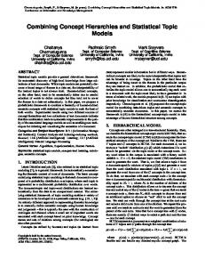
Induced concept structures were compared to those anticipated for artificial and DEX domains. For each of these, HINT converged to a single concept structure when increasing the training set size. For PALINDROME and PARITY, HINT induced expected structure of the type (x1 = x6 AND x2 = x5 ) AND (x3 = x4 ) and x1 XOR ((x2 XOR x3 ) XOR (x4 XOR x5 )). More interesting are the structures for MONK1 and MONK2. For MONK1, HINT develops a concept hierarchy (Figure 12) that (1) correctly excludes irrelevant attributes x3 , x4 , and x6 ,
26
Figure 13: The feature hierarchy discovered for MONK2. Each node gives a name of the feature and cardinality of its set of values.
Figure 14: Original (left) and discovered structure (right) for NURSERY. (2) transforms x5 to x05 by mapping four values of x5 to only two values of x05 , (3) includes an intermediate concept c and its tabular representation for x1 = x2 , and (4) relates c and x05 with a tabular representation of the OR function. In other words, the resulting hierarchy correctly represents the target concept. For MONK2, although the discovered structure (Figure 13) does not directly correspond to the original concept definition, it correctly reformulates the target concept by introducing concepts that count the number of ones in their arguments. Also note that all attributes that have more than two values are replaced by new binary ones. For all DEX domains HINT converged to concept hierarchies that were very similar to original DEX models. A typical example is NURSERY, for which Figure 14 shows the original DEX model and the concept hierarchy discovered by HINT. Note that the two structures are actually the same except that some original DEX intermediate concepts were additionally decomposed. Similarities of the same type were also observed for other DEX domains. For NURSERY, no attributes were removed by preprocessing and redundancies were found only in attributes’ domains: applicant’s social status none and medium were found equivalent, 27
and there was no difference between a family having 3 or more-than-3 children. Similar type of redundancies were also found in other DEX models. When a decision support expert that participated in the development of DEX models was asked to comment on these findings, he indeed recognized most of them as those that were intentionally used in DEX models with future extension and specialization of model functions in mind.
6.4
Comparison of partition selection measures
So far, all experiments with HINT used column multiplicity as the partition selection measure. The same experiments were also performed under the same settings but using two informationbased partition selection measures. The study revealed that there are no significant differences in terms of classification accuracy. Figure 15 depicts typical examples of learning curves; only average classification accuracies are shown, which are for all training set sizes insignificantly different for all three measures. Moreover and especially for artificial and DEX datasets, HINT converged to the same concept structure for either of the selection measures. To conclude, it is interesting that a measure as simple as column multiplicity performed equally well as the other two more complex measures.
100
� ∗
∗ ∗ � � � ∗ ∗ � ∗ � ∗ � � � ∗ ∗
..... .................. ............. ............4 . ...4 ........ ...... . ..4 ....... ...... ........... .......4 .........4 ...... ... ......... ........ ... .... .4 ............ .....4 ..... . . . . . . ............ . ...4 .. ..... ...... 4 ..... ........... ..... .... ........ 4
75
� ∗
� ∗ � ∗ � ∗ ∗ �
... ..........4 ..............4 .............4 ....................... .4 ................. 4 ........... ...... .......... ...4 .... .................... 4 . . . ... ... ........ ........ 4 ... ... ...... . . ... ... ... ... 4 ... ... .... .... .. .. ... .. ....... ........ ..... ....... ..... 4
100
∗ ∗ � �
∗ � ∗ � ∗ ∗ � � ∗ �
... ..............4 .............4 ............4 ....................... .....4 ....... ... 4 ........... .... ... . . . . . ......... ......4 4 ...... ..... ... .... .. ...... . ....... ...... .... ... . 4 . . ..... ..... ..... ....... .4 . . . .. .. ... . ... ..... 4 ... . . . ....
100
∗ �
� ∗
75
� ∗
� ∗
75
� ∗
� ∗
∗ �
� ∗
50
50 0
20
40
60
80
100
0
20
(a) PROMOTERS
40
60
80
100
0
4
∗ ψs
ψν
20
40
60
80
100
(c) BREAST
(b) HOUSING
Legend:
∗ �
50
4
ψc
Figure 15: Learning curves for different partition selection measures.
7
Related work
The decomposition approach to machine learning was used early by a pioneer of artificial intelligence, A. Samuel. He proposed a method based on a signature table system [44] and used it as an evaluation mechanism for his checkers playing programs. A signature table system is a tree of input, intermediate, and a single output variable, and is essentially an identical representation of concept trees as used in this article. Signature tables define the 28
intermediate concepts and use signatures (examples) that completely cover the attribute space. The value of an output variable is determined by a bottom-up derivation that first assigns the values to the intermediate variables, and finally derives the value of the output variable. Samuel used a manually defined concept structures with two layers of intermediate concepts. Learning was based on presenting a set of book moves to the concept hierarchy and adjusting the output values of the signatures according to the correlation coefficient computed from learning examples. Compared to his previous approach that was based on the learning of the coefficients in a linear evaluation polynomial [43], Samuel showed that the use of a signature table system significantly improves the performance. Samuel’s approach was later studied and improved by Biermann et al. [2], but still required the concept structure to be given in advance. While, within machine learning, Samuel and Biermann et al. may be the first to realize the power of using concept hierarchies, fundamentals of the approach that can discover such hierarchies were defined earlier in the area of switching circuit design. Curtis [10] reports that in the late 1940’s and 1950’s several switching circuit theorists considered this subject and in 1952 Ashenhurst reported on a unified theory of decomposition of switching functions [1]. The method proposed by Ashenhurst decomposes the truth table of a Boolean function to be realized with standard binary gates. Most of other related work of that time is reported and reprinted in [10], where Curtis compares the decomposition approach to other switching circuit design approaches and further formalizes and extends the decomposition theory. Besides a disjoint decomposition, where each variable can appear as input in just one of the derived tables, Curtis defines a non-disjoint decomposition where the resulting structure is an acyclic graph rather than a tree. Furthermore, Curtis defines a decomposition algorithm that aims at constructing a switching circuit of the lowest complexity, i.e., with the lowest number of gates used. Curtis’ method is defined over two-valued variables and requires a set of examples that completely cover the attribute space. Recently, the Ashenhurst-Curtis approach was substantially improved by research groups of M. A. Perkowski, T. Luba, and T. D. Ross. Perkowski and Uong [34] and Wan and Perkowski [50] propose a graph coloring approach to the decomposition of incompletely specified switching functions. A different approach is presented by Luba and Selvaraj [23]. Their decomposition algorithms are able to generalize. A generalization of function decomposition when applied to a set of simple Boolean functions was studied by Ross et al. [40] and Goldman [14]. The authors indicate that the decomposition approach to switching function design may be termed knowledge discovery as functions and features not previously anticipated can be discovered. A similar point, but using different terminology, was made already by Curtis [10], who observed that the same truth table representing a Boolean function might have different decompositions. Feature discovery has been at large investigated by constructive induction, a recently active field within machine learning. The term was first used by Michalski [25], who defined it 29
as an ability of the system to derive and use new attributes in the process of learning. Following this idea and perhaps closest to function decomposition are the constructive induction systems that use a set of constructive operators to derive new attributes. Examples of such systems are described in [24, 35, 38]. The main limitation of these approaches is that the set of constructive operators has to be defined in advance. Moreover, in constructive induction, the new features are primarily introduced for the purpose of improving the classification accuracy of the induced classifier, while the above described function decomposition approaches focused primarily on the reduction of complexity, where the impact on classification accuracy can be regarded rather as a side-effect of decomposition-based generalization. In first-order learning of relational concept descriptions, constructive induction is referred to as predicate invention. An overview of recent achievements in this area can be found in [47]. Decomposition with nominal-valued attributes and classes may be regarded as a straightforward extension of Ashenhurst-Curtis approach. Such an extension was described by Biermann et al. [2]. Alternatively, Luba [22] proposes a decomposition where multi-valued intermediate concepts are binarized. Files et al. [13] propose a decomposition approach for k-valued logic where both attributes and intermediate concepts take at most k values. A concept structure as used in this article defines a declarative bias over the hypothesis space. Biermann et al. [2] showed that concept structure significantly limits the number of representable functions. This was also observed by Russel [41], who proved that treestructured bias can reduce the size of concept language from doubly-exponential to singly exponential in the number of attributes. Tadepalli and Russel [48] show that such bias enables PAC-learning of tabulated functions within concept structure. Their approach for decomposition of Boolean functions requires the concept structure to be given in advance. Their learning algorithm differs from the function decomposition approaches in that it uses both examples and queries, i.e., asks the oracle for the class value of instances that are needed in derivation but not provided in the training examples. Similar to function decomposition, the learning algorithm of Tadepalli and Russel induces intermediate concepts that are lower in the hierarchy first. As with Ashenhurst-Curtis decomposition, the resulting classifiers are consistent with training examples. Queries are also used in PAC-learning described by Bshouty et al [8]. Their algorithm identifies both concept structures and their associated tabulated functions, but can deal only with Boolean functions with symmetric and constant fan-in gates. Within PAC-learning, Hancock et al. [16] learn non-overlapping perceptron networks from examples and membership queries. An excellent review of other related work in PAC-learning that uses structural bias and queries is given in [48]. Function decomposition is also related to construction of oblivious read-once decision graphs (OODG). OODGs are rooted, directed acyclic graphs that can be divided into levels [17]. All nodes at a level test the same attribute, and all edges that originate from one level terminate at the next level. Like with decision trees, OODG leaf nodes represent class values. OODGs can be regarded as a special case of decomposition, where decomposition structures 30
are of the form f1 (x1 , f2 (x2 , . . . , fn (xn ))) and where xn is at the top of a decision graph and the number of nodes at each level equals the number of distinct output values used by corresponding function fi . In fact, decision graphs were found as a good form of representation of examples to be used by decomposition [21, 20, 13]. Within machine learning, the use of oblivious decision graphs was studied by Kohavi [17]. Graphs induced by his learning algorithm are consistent with training examples, and for incomplete datasets the core of the algorithm is a graph coloring algorithm similar to the one defined by Perkowski and Uong [34]. Of other machine learning approaches that construct concept hierarchies we here mention Muggleton’s DUCE [29, 30] which uses transformation operators to compress the given examples by successive generalization and feature construction. Nevill-Manning and Witten [32] describe SEQUITUR, an algorithm that infers a hierarchical structure from a sequence of discrete symbols. Although there are some similarities with function decomposition (e.g., maintaining consistency and induction of new features), DUCE and SEQUITUR are essentially different in both the algorithmic and representational aspects. Within machine learning, there are other approaches based on problem decomposition, but where the problem is decomposed by an expert and not discovered by a machine. A wellknown example is structured induction, a term introduced by Donald Michie and applied by Shapiro and Niblett [46] and Shapiro [45]. Their approach is based on a manual decomposition of the problem and an expert-assisted selection and classification of examples to construct rules for intermediate concepts in the hierarchy. In comparison with standard decision tree induction techniques, structured induction exhibits about the same classification accuracy with the increased transparency and lower complexity of the developed models. Michie [26] emphasized the important role of structured induction in the future and listed several real problems that had been solved in this way. Mozetiˇc [27, 28, 7] employed another scheme for structuring the learning problem. That approach was particularly aimed at automated construction of system models from inputoutput observations of the system’s behavior. The structure of the learning problem, specified by a Prolog clause, corresponded to the physical structure of the modeled system in terms of the system’s components and connections among them. In an experiment, a substantial part of a qualitative model of the heart was induced from examples of the behavior of the heart. It was shown that the structuring of the domain very significantly improved the effectiveness of learning compared to unstructured learning. Again, the structure of the system was specified by the user and not induced automatically. Concept hierarchy has also been used in a multi-attribute decision support expert system shell DEX [6] which has its roots in DECMAK methodology [12, 3]. There, a tree-like structure of variables is defined by an expert, and several tools assist in the acquisition of decision rules. These are, like Samuel’s signature tables, used to derive the values of intermediate and output variables. DEX also allows different representations of user-defined decision tables, including decision trees [45] and decision rules [39]. DEX has been applied in 31
more than 50 real decision making problems. The method presented in this article essentially borrows from three different research areas: it shares the motivation with structured induction and structured approach to decision support, while the core of the method is based on Ashenhurst-Curtis function decomposition. In comparison with related work, the present article is original in the following respects: new method for handling multi-valued attributes and classes, improved decomposition heuristics, treatment of redundancies, emphasis on generalization effects of decomposition, paying strong attention to the discovery of meaningful concept hierarchies, and experimental evaluation on machine learning problems. Our earlier experiments in function decomposition applied to DEX domains were presented in [54, 53].
8
Conclusion
We introduced a new machine learning approach based on function decomposition. A distinguishing feature of this approach is its capability to discover new intermediate concepts, organize them into a hierarchical structure, and induce the relationships between the attributes, newly discovered concepts, and the target concept. In their basic form, these relationships are specified by newly constructed example sets. In a way, the learning process can thus be viewed as a process of generating new, equivalent example sets, which are consistent with the original example set. The new sets are smaller, have smaller number of attributes, and introduce intermediate concepts. Generalization also occurs in this process. We have evaluated the decomposition-based learning method on several datasets. In particular, we studied the accuracy of the induced descriptions by HINT and its capability to discover meaningful hierarchies. For all datasets where useful hierarchies existed, HINT significantly outperformed C4.5 and found relevant concept hierarchies, provided that enough examples were used for training. Experiments show that decomposition is more sensitive to undersampling and, especially in more complex datasets, C4.5 performed relatively better with small training sets. For other datasets, with no useful concept structure, C4.5 and HINT performed similarly in all but one domain. In terms of the meaningfulness of discovered structures, the most significant experiments were those with DEX domains. For these domains HINT’s task was to reconstruct the underlying concept hierarchy. We have observed that for all six domains investigated, HINT converges to concept hierarchies that are very similar or identical to those anticipated. It should be emphasized that we consider these similarities of concept structures as the most significant indicator of HINT’s success. The approach described in this article is limited to consistent datasets and nominal features. It is therefore desired to extend the approach to discover new features from noisy data, and from data that comprises continuous features. To handle noisy data, a minimal-error decomposition was recently proposed [52]. It is based on a representation of training examples 32
with class distributions and uses successive column merging of partition matrix, so that the expected error of classification is minimized. For continuously-valued datasets, the function decomposition method was proposed in [11]. They both present preliminary results which strongly encourage further development in this direction and integration of their techniques into common function decomposition framework. The feature construction aspect of HINT is investigated in more detail in [55].
References [1] R. L. Ashenhurst. The decomposition of switching functions. Technical report, Bell Laboratories BL-1(11), pages 541–602, 1952. [2] A. W. Biermann, J. Fairfield, and T. Beres. Signature table systems and learning. IEEE Trans. Syst. Man Cybern., 12(5):635–648, 1982. [3] M. Bohanec, I. Bratko, and V. Rajkoviˇc. An expert system for decision making. In H. G. Sol, editor, Processes and Tools for Decision Support. North-Holland, 1983. [4] M. Bohanec, B. Cestnik, and V. Rajkoviˇc. A management decision support system for allocating housing loans. In P. Humphreys, L. Bannon, A. McCosh, and P. Migliarese, editors, Implementing System for Supporting Management Decisions, pages 34–43. Chapman & Hall, London, 1996. [5] M. Bohanec and V. Rajkoviˇc. Knowledge acquisition and explanation for multi-attribute decision making. In 8th Intl Workshop on Expert Systems and their Applications, pages 59–78, Avignon, France, 1988. [6] M. Bohanec and V. Rajkoviˇc. DEX: An expert system shell for decision support. Sistemica, 1(1):145–157, 1990. [7] I. Bratko, I. Mozetiˇc, and N. Lavraˇc. KARDIO: a study in deep and qualitative knowledge for expert systems. MIT Press, 1989. [8] N. H. Bshouty, T. R. Hancock, and L. Hellerstein. Learning boolean read-once formulas over generalized bases. Journal of Computer and System Sciences, 50(3):521–542, 1995. [9] T. H. Cormen, C. E. Leiserson, and R. L. Rivest. Introduction to Algorithms. MIT Press, 1989. [10] H. A. Curtis. A New Approach to the Design of Switching Functions. Van Nostrand, Princeton, N.J., 1962. [11] J. Demˇsar, B. Zupan, M. Bohanec, and I. Bratko. Constructing intermediate concepts by decomposition of real functions. In M. van Someren and G. Widmer, editors, Proc. European Conference on Machine Learning, ECML-97, pages 93–107, Prague, April 1997. Springer. [12] J. Efstathiou and V. Rajkoviˇc. Multiattribute decisionmaking using a fuzzy heuristic approach. IEEE Trans. on Systems, Man and Cybernetics, 9:326–333, 1979. [13] C. Files, R. Drechsler, and M. Perkowski. Functional decomposition of MVL functions using multi-valued decision diagrams. In International Symposium on Multi-Valued Logic, may 1997.
33
[14] J. A. Goldman. Pattern theoretic knowledge discovery. In Proc. the Sixth Int’l IEEE Conference on Tools with AI, 1994. [15] R. L. Graham, D. E. Knuth, and O. Patashnik. Concrete mathematics: a foundations for computer science. Addison-Wesley, 1994. [16] T. R. Hancock, M. Golea, and M. Marchand. Learning nonoverlaping perceptron networks from examples and membership queries. Machine Learning, 16(3):161–183, 1994. [17] R. Kohavi. Bottom-up induction of oblivious read-once decision graphs. In F. Bergadano and L. De Raedt, editors, Proc. European Conference on Machine Learning, pages 154–169. Springer– Verlag, 1994. [18] I. Kononenko. Estimating attributes. In F. Bergadano and L. De Raedt, editors, Proc. of the European Conference on Machine Learning (ECML-94), pages 171–182. Springer-Verlag, 1994. ˇ ˇ [19] I. Kononenko, E. Simec, and M. Robnik Sikonja. Overcoming the myopia of inductive learning algorithms with ReliefF. Applied Intelligence Journal, 7(1):39–56, 1997. [20] Y.-T. Lai, K.-R. R. Pan, and M. Pedram. OBDD-based function decomposition: Algorithms and implementation. IEEE Transactions on Computer Aided Design of Integrated Circuits and Systems, 15(8):977–990, 1996. [21] Y.-T. Lai, M. Pedram, and S. Sastry. BDD-based decomposition of logic functions with application to FPGA synthesis. In 30th DAC, pages 642–647, 1993. [22] T. Luba. Decomposition of multiple-valued functions. In 25th Intl. Symposium on Multiple-Valued Logic, pages 256–261, Bloomigton, Indiana, May 1995. [23] T. Luba and H. Selvaraj. A general approach to boolean function decomposition and its application in FPGA-based synthesis. VLSI Design, 3(3–4):289–300, 1995. [24] R. S. Michalski. A theory and methodology of inductive learning. In R. Michalski, J. Carbonnel, and T. Mitchell, editors, Machine Learning: An Artificial Intelligence Approach, pages 83–134. Kaufmann, Paolo Alto, CA, 1983. [25] R. S. Michalski. Understanding the nature of learning: Issues and research directions. In R. Michalski, J. Carbonnel, and T. Mitchell, editors, Machine Learning: An Artificial Intelligence Approach, pages 3–25. Kaufmann, Los Atlos, CA, 1986. [26] D. Michie. Problem decomposition and the learning of skills. In N. Lavraˇc and S. Wrobel, editors, Machine Learning: ECML-95, Notes in Artificial Intelligence 912, pages 17–31. Springer-Verlag, 1995. [27] I. Mozetiˇc. Learning of qualitative models. In I. Bratko and N. Lavraˇc, editors, Progress in Machine Learning. Sigma Press, 1987. Wilmslow, England. [28] I. Mozetiˇc. The role of abstractions in learning of qualitative models. In Proc. Fourth Int. Workshop on Machine Learning. Morgan Kaufmann, 1987. Irvine, Ca. [29] S. Muggleton. Structuring knowledge by asking questions. In I. Bratko and N. Lavraˇc, editors, Progress in Machine Learning, pages 218–229. Sigma Press, 1987.
34
[30] S. Muggleton. Inductive Acquisition of Expert Knowledge. Addison-Wesley, Workingham, England, 1990. [31] P. M. Murphy and D. W. Aha.
UCI Repository of machine learning databases [http://www.ics.uci.edu/~mlearn/mlrepository.html]. Irvine, CA: University of California, Department of Information and Computer Science, 1994.
[32] C. G. Nevill-Manning and I. H. Witten. Identifying hierarchical structure in sequences: A lineartime algorithm. Journal of Artificial Intelligence Research, 7:67–82, 1997. [33] M. Olave, V. Rajkoviˇc, and M. Bohanec. An application for admission in public school systems. In I. Th. M. Snellen, W. B. H. J. van de Donk, and J.-P. Baquiast, editors, Expert Systems in Public Administration, pages 145–160. Elsevier Science Publishers (North Holland), 1989. [34] M. Perkowski and H. Uong. Automatic design of finite state machines with electronically programmable devices. In Record of Northcon ’87, pages 16/4.1–16/4.15, Portland, OR, 1987. [35] B. Pfahringer. Controlling constructive induction in CiPF. In F. Bergadano and L. De Raedt, editors, Machine Learning: ECML-94, pages 242–256. Springer-Verlag, 1994. [36] J. R. Quinlan. C4.5: Programs for Machine Learning. Morgan Kaufmann Publishers, 1993. [37] R. Quinlan. Induction of decision trees. Machine Learning, 1(1):81–106, 1986. [38] H. Ragavan and L. Rendell. Lookahead feature construction for learning hard concepts. In Proc. Tenth International Machine Learning Conference, pages 252–259. Morgan Kaufman, 1993. [39] V. Rajkoviˇc and M. Bohanec. Decision support by knowledge explanation. In H. G. Sol and J. Vecsenyi, editors, Environments for supporting Decision Process. Elsevier Science Publishers B.V., 1991. [40] T. D. Ross, M. J. Noviskey, D. A. Gadd, and J. A. Goldman. Pattern theoretic feature extraction and constructive induction. In Proc. ML-COLT ’94 Workshop on Constructive Induction and Change of Representation, New Brunswick, New Jersey, July 1994. [41] S. J. Russell. Tree-structured bias. In M. N. Saint Paul, editor, Proc. The Seventh National Conference on Artificial Intelligence, pages 641–645, San Mateo, CA, 1988. Morgan Kaufmann. [42] S. L. Salzberg. On comparing classifiers: Pitfalls to avoid and a recommended approach. Data Mining and Knowledge Discovery, 1:317–328, 1997. [43] A. Samuel. Some studies in machine learning using the game of checkers. IBM J. Res. Develop., 3:221–229, 1959. [44] A. Samuel. Some studies in machine learning using the game of checkers II: Recent progress. IBM J. Res. Develop., 11:601–617, 1967. [45] A. D. Shapiro. Structured induction in expert systems. Turing Institute Press in association with Addison-Wesley Publishing Company, 1987. [46] A. D. Shapiro and T. Niblett. Automatic induction of classificiation rules for a chess endgame. In M. R. B. Clarke, editor, Advances in Computer Chess 3, pages 73–92. Pergamon, Oxford, 1982. [47] I. Stahl. An overview of predicate invention techniques in ILP. In ESPRIT BRA 6020: Inductive Logic Programming, 1991.
35
[48] P. Tadepalli and S. Russell. Learning from examples and membership queries with structured determinations. Machine Learning (to appear). [49] S. B. Thrun et al. A performance comparison of different learning algorithms. Technical report, Carnegie Mellon University CMU-CS-91-197, 1991. [50] W. Wan and M. A. Perkowski. A new approach to the decomposition of incompletely specified functions based on graph-coloring and local transformations and its application to FPGA mapping. In Proc. of the IEEE EURO-DAC ’92, pages 230–235, Hamburg, September 1992. [51] D. J. A. Welsh and M. B. Powell. An upper bound on the chromatic number of a graph and its application to timetabling problems. Computer Journal, 10:85–86, 1967. [52] B. Zupan. Machine learning based on function decomposition. PhD thesis, University of Ljubljana, April 1997. Available at http://www-ai.ijs.si/BlazZupan/papers.html. [53] B. Zupan, M. Bohanec, I. Bratko, and B. Cestnik. A dataset decomposition approach to data mining and machine discovery. In D. Heckerman, H. Mannila, D. Pregibon, and R. Uthurusamy, editors, Proc. of the Third International Conference on Knowledge Discovery and Data Mining (KDD-97), pages 299–303, Irvine, CA, August 1997. AAAI Press. [54] B. Zupan, M. Bohanec, I. Bratko, and J. Demˇsar. Machine learning by function decomposition. In Jr. D. H. Fisher, editor, Proc. Fourteenth International Conference on Machine Learning (ICML97), pages 421–429, San Mateo, CA, 1997. Morgan Kaufmann. [55] B. Zupan, M. Bohanec, J. Demˇsar, and I. Bratko. Feature transformation by function decomposition. IEEE Intelligent Systems & Their Applications, 13(2):38–43, March/April 1998.
36