Learning Efficient Rules by Maintaining the Explanation Structure Jihie Kim and Paul S. Rosenbloom Information Sciences Institute and Computer Science Department University of Southern California 4676 Admiralty Way Marina del Rey, CA 90292, U.S.A.
[email protected],
[email protected]
Abstract Many learning systems suffer from the utility problem; that is, that time after learning is greater than time before learning. Discovering how to assure that learned knowledge will in fact speed up system performance has been a focus of research in explanationbased learning (EBL). One way to analyze the utility problem is by examining the differences between the match process (match search) of the learned rule and the problem-solving process from which it is learned. Prior work along these lines examined one such difference. It showed that if the search-control knowledge used during problem solving is not maintained in the match process for learned rules, then learning can engender a slowdown; but that this slowdown could be eliminated if the match is constrained by the original search-control knowledge. This article examines a second difference — when the structure of the problem solving differs from the structure of the match process for the learned rules, time after learning can be greater than time before learning. This article also shows that this slowdown can be eliminated by making the learning mechanism sensitive to the problem-solving structure; i.e., by reflecting such structure in the match of the learned rule.
Introduction Efficiency is a major concern for all problem solving systems. One way of achieving efficiency is the application of learning techniques to speed up problem solving. Explanation-based learning (EBL)(Mitchell, Keller, & Kedar-Cabelli 1986; DeJong & Mooney 1986) can improve performance by acquiring new search-control rules 1 . Given its four informational components — the goal concept, the training example, the domain theory, and the operationality criterion — EBL generates a new search control rule that is intended to reduce the search required in subsequent problems. Unfortunately, EBL suffers from the utility problem, so that the cost of using learned rules often overwhelms their benefit. Research on the utility problem can be divided up into 1
EBL can also be used to acquire other types of structures, such as macro-operators, but we focus on search-control rules here.
two key issues. The first issue is the expensive chunk 2 problem (Tambe 1991), in which individual learned rules are so expensive to match that the system suffers a slow down from learning (Minton 1988; Tambe 1991; Etzioni 1990; Shell & Carbonell 1991; Subramanian & Feldman 1990). The second issue is the average growth effect (Doorenbos, Tambe, & Newell 1992), in which the interactions across the rules slow down the system, even if none of the rules individually are all that expensive. Recent work on the average growth effect has shown that it is possible to learn over one million rules while still allowing their efficient use (Doorenbos, Tambe, & Newell 1992; Doorenbos 1993). In this article we focus on the expensive chunk problem. Previous work on the expensive chunk problem has investigated how to produce cheaper rules (Prieditis & Mostow 1987; Minton 1988; Shell & Carbonell 1991; Shavlik 1990; Etzioni 1990) and how to filter out expensive rules (Minton 1988; Greiner & Jurisica 1992; Gratch & Dejong 1992; Markovitch & Scott 1993). However, none of these approaches can generally guarantee that the cost of using the learned rules will always be bounded by the cost of the problem solving episode from which they are learned. That is, the cost of a learned rule can be greater than the cost of solving the problem with the original set of rules. There has been developed a technique for restricting the expressiveness of the rules to bound the match cost of the rules (Tambe 1991). However, the restriction reduces the expressibility of the rules, requiring a large number of rules to encode tasks. Also, the learned rules may become very specific. One way of finding a solution which can guarantee cost boundedness without such a restriction is to investigate the differences between the match process (i.e., the search performed during match 3 ) of the learned rule and the problem-solving process from which it is learned. By analyzing the differences, we can identify a set of sources which can make the output rule expensive. Prior work on this topic has examined one such difference: in chunking (and other EBL systems which use search control in problem solving), eliminating search control in learning can increase the cost of the learned rules (Kim & 2 Chunk means any learned rule. This is a generalization of the term used in the Soar system. 3 What is referred to as k-search in (Tambe 1991).
Rosenbloom 1993). For example, PRODIGY/EBL(Minton 1993) and Soar (Laird, Newell, & Rosenbloom 1987; Rosenbloom et al. 1991) — two problem solvers that learn rules by variants of EBL — ignore many of the searchcontrol rules during learning in order to increase the generality of the learned rules. However, the consequence of this omission is that the learned rules are not constrained by the path actually taken in the problem space, and thus can perform an exponential amount of search even when the original problem-solving search was highly directed (by the control rules). This problem was solved in (Kim & Rosenbloom 1993) by extending the explanation to include the search-control rules used during problem solving, thus creating more appropriately constrained rules. In this article, we focus on a second difference — when the structure of the problem solving differs from the structure of the match process for the learned rules, time after learning can be greater than time before learning. During problem solving, the rules that fire tend to form a hierarchical structure in which the early rules provide information upon which the firing of later rules depends. This hierarchical structure is reflected in EBL most obviously in the structure of the explanation (and the more general explanation structure). However, if this hierarchical structure is then flattened into a linear sequence of conditions for use in matching the rule that is learned — as must be done in creating Ops-like rules or Prolog clauses — the time after learning can be greater than the time before learning. If instead, the learning mechanism is made sensitive to the problem-solving structure — i.e., by reflecting such hierarchical structure in the match of the learned rule — this source of expensiveness can be avoided. The focus of the analysis in this paper is Soar/EBL (Kim & Rosenbloom 1995). Although our prior work is based on chunking(Laird, Rosenbloom, & Newell 1985) in Soar, we analyze an implementation of EBL in Soar here to be able to more easily generalize the resulting analysis to other EBL systems. Soar/EBL is a little different from the standard version of Soar with chunking. Soar/EBL creates an explanation structure (i.e., it replaces rule instantiations with rules) and employs regression in deciding which variables should be included in the learned rule, while chunking creates a new rule by directly variablizing one particular class of symbols in the explanation (i.e., in the rule instantiations).
Background In Soar, productions comprise the domain theory for Soar/EBL. Each production consists of a set of conditions and a set of actions. Conditionstest working memory for the presence or absence of patterns of tuples, where each tuple consists of an object identifier, an attribute and a value. Actions create preferences, each of which specifies the relative or absolute worth of a value for an attribute of a given object. Productions in Soar propose changes to working memory through these preferences, and do not actually make the changes themselves. Changes to working memory are made based on a synthesis of the preferences (by a fixed decision procedure). The cycle of production firings, creation
Figure 1: An example of Soar/EBL process. of preferences, and creation of working memory elements (WMEs) underlies the problem solving. In the remainder of this article, when we talk about the cost of problem solving, we will be referring to the match cost of the rules that fired plus the cost of making decisions.4 To create rules, Soar maintains an instantiated trace of the rules. The set of instantiations connected to the goal achievement becomes the proof tree (or explanation) for Soar/EBL. The instantiations in the explanation are replaced by rules which have unique names for the variables across the rules. This new structure is called the explanation structure. A regression algorithm (our algorithm is inspired by the EGGS generalization algorithm (Mooney & Bennett 1986)) is applied to this explanation structure. A set of substitutions is computed by unifying each connected actioncondition pair, and the substitutions are then applied to the variables in the explanation structure. The operational conditions become the conditions of the new rule. The action of the rule is the generalization of the goal concept. An example of Soar/EBL is shown schematically in Figure 1. The two striped vertical bars mark the beginning and the end of the problem solving. T1 – T4 are traces of the rule firings. For example, T1 records a rule firing which examined WMEs A and B and generated a preference suggesting WME G. The highlighted rule traces are those included in the explanation; T2, T3, and T4 have participated in the result creation. This explanation is generalized by regression, and a new rule is created. The match algorithm is critical in computing both the cost of problem solving and the cost of matching learned rules. Soar employs Rete as the match algorithm. When a new rule is created, it is compiled into a Rete network. Rete is one of the most efficient rule-match algorithms presently known. Its efficiency stems primarily from two key optimizations: sharing and state saving. Sharing of common conditions in a production, or across a set of productions, reduces the number of tests performed during match. State saving 4 The cost of a problem solving episode also actually includes the costs of firing rules (i.e., executing actions). However, we will not explicitly focus on this factor here because it drops out in the learning process.
Figure 2: Rete network of a rule.
preserves the previous (partial) matches for use in the future. Figure 2 illustrates a Rete network for a rule. Each WME consists of an object identifier, an attribute (indicated by a ^ ), and a value. Symbols enclosed in angle brackets are variables. The conditions of the rule are compiled into a data flow network. Rete requires a total ordering on the conditions of a rule for it to be compiled, so the rule’s conditions are first ordered by a heuristic algorithm before the rule is compiled. For example, the conditions in Figure 2 are ordered (C1, C2, C3). The network has two parts. The alpha part performs constant tests on WMEs, such as tests for at and yes. The output of these tests is stored in alpha memories. Each alpha memory contains the set of WMEs which pass all of the constant tests of a condition (or more than one, if it is shared). The beta part of the network contains join nodes and beta memories.5 Join nodes perform consistency tests on variables shared between the current condition and earlier conditions, such as , which is shared between C1 and C2. Beta memories store partial instantiations of productions; that is, instantiations of initial subsequences of conditions. The partial instantiations are called tokens. Because match time per token is known to be approximately constant in Rete (Tambe et al. 1988; Tambe 1991) — and because counting tokens yields a measure that is independent of machines, optimizations, and implementation details — we will follow the standard practice established within the match-algorithm community and use the number of tokens as a comparative measure of match cost in addition to time. 5
There also are negative nodes, into which negative conditions are compiled. A negative node passes a partial instantiation when there are no consistent WMEs.
Figure 3: Loss of independence by linearization.
A Source of Expensiveness: Linearization As mentioned briefly in the previous section, after the explanation structure is regressed, the set of operational conditions are compiled into a Rete network for future matches of the learned rule. In the process, the hierarchy in the explanation structure (which reflects the structure of the rule firings during problem solving) is linearized into a total ordering and then conditions are reordered via a heuristic algorithm to improve the match performance. The critical consequence of this step (linearization and condition ordering) is that the match structure of the learned rule is no longer constrained by the search structure of the problem solving. That is, how instantiations of different conditions are combined can be different from how they were combined during the problem solving. This structural change introduces four different sources of expensiveness. The first source arises directly from the linearization of the hierarchical structure. By combining sub-hierarchies together, some of the previously independent conditions get joined with other parts of the structure before they finish their sub-hierarchy match. Figure 3 shows an example. The problem-solving structure in Figure 3-(b) shows the rule firing structure during the problem solving, given the WMEs and rules in Figure 3-(a). The number in front of each node indicates the number of tokens (partial instantiations) at that condition. The total number of tokens in the match for the rule is the sum of these numbers (43 in this
Figure 4: Loss of sharing by linearization. case). In the problem-solving structure, the conditions in a sub-hierarchy (e.g., the conditions in R1) are matched independently from the other parts of the structure (e.g., the conditions of R2) before its created WMEs are joined with the WMEs created by R2. By combining these sub-hierarchies together — through linearization — some of these previously independent conditions get joined with other parts of the structure before they finish their sub-hierarchy match. In Figure 3-(c), it is no longer possible to maintain independence between the conditions of R1 and R2. For example, in the first case, tokens for the conditions from R2 — (
^ z ) and ( ^ u ) — are dependent on tokens for the conditions of R1. This loss of independence can increase the number of tokens. For the three orderings shown in Figure 3-(c), the number of tokens for the linearized structures are 50, 48, and 64, which are all greater than 43. No matter what condition ordering is used, the number of tokens still increases, given the WMEs in Figure 3-(a). The second source of cost increase is loss of sharing. As long as Rete cannot capture the sharing from the nonlinear structure, the number of tokens can increase. Figure 4 shows an example. Given the rules in Figure 4-(a), the problem solving shares the instantiations of R1 for both conditions C2 and C4 of rule R2. That is, they match the WMEs created from the instantiations of R1. (The total number of tokens is 15 in the problem solving.) Although the instantiations are shared, C2 and C4 are matched by different WMEs because and cannot be bound to the same value (given the initial set of WMEs in Figure 4-(a)). So, two instantiations of R1 participate in the explanation; one of them creates the WME matched by C2,
Figure 5: Non-optimal ordering can increase the cost.
and the other creates the WME matched by C4. Figure 4-(c) shows the explanation structure generated from the explanation. R1 is separated into R1’ and R1”, by replacing the two instantiations with two rules. The learned rule (with an optimal ordering) from the explanation structure is shown in Figure 4-(d). The total number of tokens is increased from 15 to 19. This increase stems from the linearization rather than having separate copies for each instantiation in the explanation, because a smart compiler of the structure in Figure 4-(c) may still share R1’ and R1”. The two have the same structure and the same pattern of consistency tests across the conditions, and they can be compiled into the same structure. By linearization, this sharing becomes impossible. The third source of cost increase comes from non-optimal ordering of the conditions. Finding an optimal ordering for a set of conditions can take as the factorial in the number of conditions (considering all possible orderings), and Rete employs a heuristic ordering algorithm. Because the heuristic condition-ordering algorithm cannot guarantee optimal orderings, whenever this algorithm creates a non-optimal ordering, additional cost may be incurred. For example, given the WMEs and rules in Figure 5-(a), the total number of tokens in the problem solving is 15 (Figure 5-(b)). While the cost can be reduced to 10 by an optimal ordering (as shown in Figure 5-(c)), a non-optimal ordering can increase it to 16 (as shown in Figure 5-(d)). The fourth source of cost increase is inefficient searchcontrol combination. The previous work on incorporating search control in the explanation has shown that search control can constrain the match process of learned rules by
Figure 6: Extending the proof structure to capture the search control rules. cutting down the search space in match and so reduce the cost. By including the search-control rules in the explanation, the proof structure is extended as shown in Figure 6. The decision nodes in Figure 6-(b) represent participation by the decision procedure in the problem solving. The integration of the search control (a set of preferences) by the decision procedure is implemented as a C function in Soar. The decision procedure filters out the rejected candidates in time linear in the number of preferences. By linearization, the structure in Figure 6-(b) is collapsed into a totally ordered structure, ignoring the decision nodes in the explanation structure. The integration of search control is transformed into an integration operation of this linear structure. The only integration operation in Rete is Join. Join nodes perform consistency tests on variables shared between the current condition and earlier conditions, and create tokens (i.e. instantiations of initial subsequences of conditions). By using this operation only, time can grow as the factorial of the number of preferences, because it creates a token for each possible ordering of the search control. Figure 7-(c) shows an example. Given the three reject conditions, six (3!) instantiations are created even with the best possible ordering of the conditions. The total number of tokens is 21. This difference between linear and factorial processes can increase the cost. Our solution to the first three problems is not to linearize conditions. By not linearizing, the first and third problems disappear. The second problem is automatically solved by Rete’s sharing. For example, R1’ and R1” in Figure 4(c) can be shared in the Rete as the conditions are shared across the rules. For the fourth problem, we introduce a new type of rete node called a decision sub-node in the nonlinear network. The node picks one of the instantiations of the conditions arbitrarily instead of keeping all of the instantiations. This ’pick one’ operation filters out rejected candidates one at a time, as the decision procedure filters a rejected candidate per preference. A sequence of decision sub-nodes produces a maximum of one token per node, and the total number of tokens is the same as the number of conditions. For instance, in case of Figure 7-(d), the join nodes for the three reject conditions are replaced by decision subnodes. The number of tokens created by this modification is one for each condition. Only one instantiation is generated instead of six (3!) instantiations. The total number of token is 4 instead of 21.
Figure 7: Tokens with linear and nonlinear match.
Figure 8: Grid task.
Experimental Results In order to supplement the analysis provided in the previous section with experimental evidence, we have extended the current Rete implementation to interpret nonlinear structure. Also, we have introduced decision sub-nodes into Rete. We have applied the resulting experimental system to the Grid task (Tambe 1991) (Figure 8), which is one of the known expensive-chunk tasks. The results shown here are all from Soar6 (version 6.0.4), a C-based release of Soar (Doorenbos 1992) on a Sun SPARCstation-20. Each problem in the Grid task is to find a path between two points in a two dimensional grid. For example, finding a path from point F to point O is a Grid task. Because F is connected to four adjacent points, four operators can be suggested by rule operator-goto-loc, as shown in Figure 8-(b). For experimental efficiency, the results presented here assume a
Grid Task
average CPU time (sec)
Without learning
0.46
Linear rule learning
1.42
Non-linear rule learning
0.34
Table 1: Average CPU time for a sequence of Grid tasks.
Figure 10: Magic Square task. Magic Task Without learning Linear rule learing Non-linear rule learning
average CPU time 4.51 — 0.50
Table 2: Average CPU time for a sequence of Magic Square tasks.
Figure 9: Number of tokens of a linear and a nonlinear learned rule in a Grid task. 10x10 bounded grid instead of an unbounded grid. All Grid tasks used here are searches for paths of length three. We compared the CPU time of three different versions of a system solving Grid tasks: problem solving time without learning, problem solving time with linear learned rules, and problem solving time with nonlinear learned rules. Table 1 shows the average CPU time per problem (in seconds), for a sequence of twelve different problems in the Grid task. Both linear-rule learning and nonlinear-rule learning systems incorporated the search control in the explanation. The average CPU time with linear-rule learning is more than three times greater than the average CPU time of the system without learning. However, the time with nonlinear learning is less than the time before learning. Figure 9 shows the number of tokens at each condition for a learned rule match in a Grid task. In linear match (Figure 9-(a)), there are huge combinations, with a maximum number of 2916, between the conditions. In the nonlinear match case, as shown in Figure 9-(b), the number does not grow to more than 4. In Figure 9-(b), braces mark the beginning and ending of a sub-part in the nonlinear match. This hierarchical structure reflects the explanation structure created from the problem solving. Shared sub-parts are not shown in the figure for brevity. The shared condi-
tions across the different sub-parts reflect the multiple usage of those conditions in the original problem solving. This multiple usage keeps the cost bounded by constraining the sub-parts as they were in the problem solving. We also applied the system to the Magic Square task(Tambe 1991) (Figure 10), another known expensivechunk task. The task involves placing tiles 1 through 9 in empty squares one at a time. If the sums of horizontal, vertical, and diagonal lines are different in the current tile placement, the task fails. Otherwise, the task succeeds. We divided the Magic Square task into nine sub-problems, each of which is the task of placing the next tile in the correct cell, given the earlier placements of tiles. Table 2 shows the average CPU time per sub-problem (in seconds) for the sequence of nine sub-problems in the Magic Square task. With linear-rule learning, the system could not even finish learning for the first sub-problem. The number of tokens for the learned rule became over eight million and the system could not allocate enough memory. The CPU time with nonlinear-rule learning is bounded by the time without learning. The time without learning is greater than the time with nonlinear-rule learning by a factor of nine.
Summary and Discussion The cost increase of using learned knowledge can be analyzed by examining the difference between the match process (match search) of learned rules and the problem-solving process from which they are learned. In this context, (Kim & Rosenbloom 1993) examined an approach that is based on incorporating search-control knowledge into the learned rule. That analysis showed that omitting search control in learning (i.e., in the explanation) can increase the cost of learned rules. The consequence of this omission is that the learned rules are not constrained by the path actually taken in the problem space, and thus can perform an exponential amount of search even when the original problem-space search was highly directed (by the control rules). (Kim
& Rosenbloom 1993) extended the explanation to include search-control rules, thus creating more constrained rules. Here we have found that even with the search-control rules incorporated in the explanation, if the system ignores the hierarchical structure in the explanation structure while matching the of learned rules, cost can still increase. 6 There are at least four causes of cost increase that arise from linearizing conditions without considering the problem-solving structure: 1. Loss of independence: By combining sub-hierarchies together through linearization, some previously independent conditions get joined with other parts of the structure before they finish their sub-hierarchy match. This change can increase the number of tokens. 2. Loss of sharing: By losing sharing that existed in the problem-solving structure, the number of tokens can increase. 3. Non-optimal reordering: The heuristic conditionordering algorithm cannot guarantee optimal orderings, which can lead to increased search. 4. Inefficient search control combination: A simple linear network cannot efficiently process the search control that participates in the explanation structure. By extending Rete to interpret nonlinear structure (with an extra type of Rete node for search-control processing), the system can avoid the sources of expensiveness. The same kind of analysis could potentially be performed for other EBL systems. By comparing the search performed during problem solving and the match search performed by the learned rule, we can identify the sources of expensiveness. Avoiding those identified sources should lead to relative boundedness in the match. (Time after learning would be bounded by time before learning.) Match algorithms are critical in computing both the cost of problem solving and the cost of matching learned rules. Rete and Treat(Miranker 1987) are the best known rule match algorithms. We performed an analysis based on Rete. We conjecture that EBL with Treat might suffer similar problems because a Treat network does not have hierarchical structure; however, we have not yet done the analysis. There has been prior work done on nonlinear match to improve sharing (Scales 1986; Tambe, Kalp, & Rosenbloom 1991; Lee & Schor 1992; Hanson & Hasan 1993). Although this work was not based on learning a new rule from problem solving, the work shares the same idea: improve the match performance by nonlinearity. One essential issue in this work is finding a general criterion for determining which form of nonlinearity is best. We expect that whenever these approaches are used in an EBL system, the explanation structure could give a clue for how to construct a nonlinear match structure. 6
The results presented in (Kim & Rosenbloom 1993) are based on chunking in Soar, not Soar/EBL. Because chunking’s rule generalization is based on the explanation (instead of the explanation structure), it can create overspecialized rules. The overspecialization of the rules can avoid part of this problem.
One negative effect of using nonlinear rules might be diminished rule readabilty. As can be seen in Figure 9-(b), the hierarchical structure is not easy to understand, even if the figure doesn’t show shared sub-parts. Even with the use of indentation to identify the hierarchy, the sharing of sub-conditions is still difficult to understand. In addition to the issues raised earlier, there are several other issues for future work. The first one is extending the experimental results to a wider range of tasks, both traditional expensive-chunks tasks and non-expensive-chunk tasks. Also, experiments on a practical domain rather than a toy domain would allow a more realistic analysis of the approach. Second, in addition to the two sources of expensiveness which have so far been found by comparing search in the problem solving and search in the match, we are working toward identifying other potential sources of expensiveness, should they exist. By finding the complete set of sources of expensiveness and avoiding those sources, the cost of using the learned rules should always be bounded by the cost of the problem solving episode from which they were learned. Finally, the approach needs to be combined with a solution to the average growth effect. The earlier work on the average growth effect in chunking has shown that it is possible to learn large number of rules without hurting overall system performance. However, because the rules created by Soar/EBL can be different from the rules created by chunking, the problem still needs to be addressed in terms of Soar/EBL.
Acknowledgments This research was supported under subcontract to the University of Southern California Information Sciences Institute from the University of Michigan, as part of contract N00014-92-K-2015 from the Advanced Systems Technology Office (ASTO) of the Advanced Research Projects Agency (ARPA) and the Naval Research Laboratory (NRL); and under contract N66001-95-C-6013 from the Advanced Systems Technology Office (ASTO) of the Advanced Research Projects Agency (ARPA) and the Naval Command and Ocean Surveillance Center, RDT&E division (NRaD). We would like to thank Jon Gratch and Milind Tambe for helpful comments on this work.
References DeJong, G. F., and Mooney, R. 1986. Explanationbased learning: An alternative view. Machine Learning 1(2):145–176. Doorenbos, B.; Tambe, M.; and Newell, A. 1992. Learning 10,000 chunks: What’s it like out there? In Proceedings of the Tenth National Conference on Artificial Intelligence, 830–836. Doorenbos, B. 1992. Soar6 release notes. Doorenbos, B. 1993. Matching 100,000 learned rules. In Proceedings of the Eleventh National Conference on Artificial Intelligence.
Etzioni, O. 1990. Why Prodigy/EBL works. In Proceedings of the Eighth National Conference on Artificial Intelligence, 916–922. Gratch, J., and Dejong, G. 1992. COMPOSER: A probabilistic solution to the utility problem in speed-up learning. In Proceedings of the Tenth National Conference on Aritificial Intelligence, 235–240. Greiner, R., and Jurisica, I. 1992. A statistical approach to solving the EBL utility problem. In Proceedings of the Tenth National Conference on Artificial Intelligence, 241–248. Hanson, E. N., and Hasan, M. S. 1993. Gator: An optimized discrimination network for active database rule condition testing. Technical Report TR-93-036, CIS Department, University of Florida. Kim, J., and Rosenbloom, P. S. 1993. Constraining learning with search control. In Proceedings of the Tenth International Conference on Machine Learning, 174–181. Kim, J., and Rosenbloom, P. 1995. Transformation analyses of learning in Soar. Technical Report ISI/RR-95-4221, Information Sciences Institute and Computer Science Department University of Southern California. Laird, J. E.; Newell, A.; and Rosenbloom, P. S. 1987. Soar: An architecture for general intelligence. Artificial Intelligence 33:1–64. Laird, J. E.; Rosenbloom, P. S.; and Newell, A. 1985. Chunking in Soar: The anatomy of a general learning mechanism. Machine Learning 1. Lee, H. S., and Schor, M. I. 1992. Match algorithms for generalized Rete networks. Artificial Intelligence 54:249– 274. Markovitch, S., and Scott, P. D. 1993. Information filtering : Selection mechanism in learning systems. Machine Learning 10(2):113–151. Minton, S. 1988. Quantitative results concerning the utility of explanation-based learning. In Proceedings of the Seventh National Conference on Artificial Intelligence, 564– 569. Minton, S. 1993. Personal communication. Miranker, D. P. 1987. Treat: A better match algorithm for AI production systems. In Proceedings of the Sixth National Conference on Artificial Intelligence, 42–47. Mitchell, T. M.; Keller, R. M.; and Kedar-Cabelli, S. T. 1986. Explanation-based generalization – a unifying view. Machine Learning 1(1):47–80. Mooney, R. J., and Bennett, S. W. 1986. A domain independent explanaion-based generalization. In Proceedings of the Fifth National Conference on Artificial Intelligence, 551–555. Prieditis, A. E., and Mostow, J. 1987. PROLEARN: Towards a Prolog interpreter that learns. In Proceedings of the Sixth National Conference on Artificial Intelligence, 494–498. Rosenbloom, P. S.; Laird, J. E.; Newell, A.; and McCarl, R. 1991. A preliminary analysis of the Soar architecture
as a basis for general intelligence. Artificial Intelligence 47(1-3):289–325. Scales, D. J. 1986. Efficient matching algorithms for the Soar/Ops5 production system. Technical Report KSL-8647, Knowledge Systems Laboratory, Department of Computer Science, Stanford University. Shavlik, J. W. 1990. Aquiring recursive and iterative concepts with explanation-based learning. Machine Learning 5:39–70. Shell, P., and Carbonell, J. 1991. Empirical and analytical performance of iterative operators. In The 13th Annual Conference of The Cognitive Science Society, 898–902. Lawrence Erlbaum Associates. Subramanian, D., and Feldman, R. 1990. The utility of EBL in recursive domain theories. In Proceedings of the Eighth National Conference on Artificial Intelligence, 942–949. Tambe, M.; Kalp, D.; Gupta, A.; Forgy, C. L.; Milnes, B. G.; and Newell, A. 1988. Soar/PSM-E: Investigating match parallelism in a learning production system. In Proceedings of the ACM/SIGPLAN Symposium on Parallel Programming: Experience with applications, languages, and systems, 146–160. Tambe, M.; Kalp, D.; and Rosenbloom, P. S. 1991. Uni-Rete: Specializing the Rete match algorithm for the unique-attribute representation. Technical Report CMUCS-91-180, School of Computer Science, Carnegie Mellon University. Tambe, M. 1991. Eliminating combinatorics from production match. Ph.D. Dissertation, Carnegie-Mellon University.