Aug 1, 1998 - ing, temporal di erence learning, evaluation functions, local search, heuristic search, simulated ..... 5.1.3 Learning Curves for Channel Routing .
Learning Evaluation Functions for Global Optimization Justin Andrew Boyan August 1, 1998 CMU-CS-98-152
School of Computer Science Carnegie Mellon University Pittsburgh, PA 15213 A dissertation submitted in partial ful llment of the requirements for the degree of Doctor of Philosophy
Thesis committee: Andrew W. Moore (co-chair) Scott E. Fahlman (co-chair) Tom M. Mitchell Thomas G. Dietterich, Oregon State University
c 1998, Justin Andrew Boyan Copyright Support for this work has come from the National Defense Science and Engineering Graduate fellowship; National Science Foundation grant IRI-9214873; the Engineering Design Research Center (EDRC), an NSF Engineering Research Center; the Pennsylvania Space Grant fellowship; and the NASA Graduate Student Researchers Program fellowship. The views and conclusions contained in this document are those of the author and should not be interpreted as representing the o�cial policies, either expressed or implied, of ARPA, NSF, NASA, or the U.S. government.
Keywords: Machine learning, combinatorial optimization, reinforcement learning, temporal di�erence learning, evaluation functions, local search, heuristic search, simulated annealing, value function approximation, neuro-dynamic programming, Boolean satis ability, radiotherapy treatment planning, channel routing, bin-packing, Bayes network learning, production scheduling
1
Abstract In complex sequential decision problems such as scheduling factory production, planning medical treatments, and playing backgammon, optimal decision policies are in general unknown, and it is often di�cult, even for human domain experts, to manually encode good decision policies in software. The reinforcement-learning methodology of \value function approximation" (VFA) o�ers an alternative: systems can learn e�ective decision policies autonomously, simply by simulating the task and keeping statistics on which decisions lead to good ultimate performance and which do not. This thesis advances the state of the art in VFA in two ways. First, it presents three new VFA algorithms, which apply to three di�erent restricted classes of sequential decision problems: Grow-Support for deterministic problems, ROUT for acyclic stochastic problems, and Least-Squares TD(�) for xed-policy prediction problems. Each is designed to gain robustness and e�ciency over current approaches by exploiting the restricted problem structure to which it applies. Second, it introduces STAGE, a new search algorithm for general combinatorial optimization tasks. STAGE learns a problem-speci c heuristic evaluation function as it searches. The heuristic is trained by supervised linear regression or Least-Squares TD(�) to predict, from features of states along the search trajectory, how well a fast local search method such as hillclimbing will perform starting from each state. Search proceeds by alternating between two stages: performing the fast search to gather new training data, and following the learned heuristic to identify a promising new start state. STAGE has produced good results (in some cases, the best results known) on a variety of combinatorial optimization domains, including VLSI channel routing, Bayes net structure- nding, bin-packing, Boolean satis ability, radiotherapy treatment planning, and geographic cartogram design. This thesis describes the results in detail, analyzes the reasons for and conditions of STAGE's success, and places STAGE in the context of four decades of research in local search and evaluation function learning. It provides strong evidence that reinforcement learning methods can be e�cient and e�ective on large-scale decision problems.
2
3
Dedication To my grandfather, Ara Boyan, 1906{93
4
5
Acknowledgments This dissertation represents the culmination of my six years of graduate study at CMU and of my formal education as a whole. Many, many people helped me achieve this goal, and I would like to thank a few of them in writing. Readers who disdain sentimentality may wish to turn the page now! First, I thank my primary advisor, Andrew Moore. Since his arrival at CMU one year after mine, Andrew has been a mentor, role model, collaborator, and friend. No one else I know has such a clear grasp of what really matters in machine learning and in computer science as a whole. His long-term vision has helped keep my research focused, and his technical brilliance has helped keep it sound. Moreover, his patience, ability to listen, and innate personal generosity will always inspire me. Unlike the stereotypical professor who has his graduate students do the work and then helps himself to the credit, Andrew has a way of listening to your half-baked brainstorming, reformulating it into a sensible idea, and then convincing you the idea was yours all along. I feel very lucky indeed to have been his rst Ph.D. student! My other three committee members have also been extremely helpful. Scott Fahlman, my co-advisor, helped teach me how to cut to the heart of an idea and how to present it clearly. When my progress was slow, Scott always encouraged me with the right blend of carrots and sticks. Tom Mitchell enthusiastically supported my ideas while at the same time asking good, tough questions. Finally, Tom Dietterich has been a wonderful external committee member|from the early stages, when his doubts about my approach served as a great motivating challenge, until the very end, when his comments on this document were especially thorough and helpful. Three friends at CMU|Michael Littman, Marc Ringuette, and Je� Schneider| also contributed immeasurably to my graduate education by being my regular partners for brainstorming and arguing about research ideas. I credit Michael with introducing me to the culture of computer science research, and also thank him for his extensive comments on a thesis draft. Only in the past year or two have I come to appreciate how amazing a place CMU is to do research. I would like to thank all my friends in the Reinforcement Learning group here, especially Leemon Baird, Shumeet Baluja, Rich Caruana, Scott Davies, Frank Dellaert, Kan Deng, Geo� Gordon, Thorsten Joachims, Andrew McCallum, Peter Stone, Astro Teller, and Belinda Thom. Special thanks also go to my o�cemates over the years, including Lin Chase, Fabio Cozman, John Hancock, and Jennie Kay. The CMU faculty, too, could not have been more supportive. Besides my committee members, the following professors all made time to discuss my thesis and assist
6 my research: Avrim Blum, Jon Cagan, Paul Heckbert, Jack Mostow, Steven Rudich, Rob Rutenbar, Sebastian Thrun, Mike Trick, and Manuela Veloso. I would also like to thank the entire Robotics Institute for allowing me access to over one hundred of their workstations for my 40,000+ computational experiments! The third major part of what makes the CMU environment so amazing is the excellence of the department administration. I would particularly like to thank Sharon Burks, Catherine Copetas, Jean Harpley, and Karen Olack, who made every piece of paperwork a pleasure (well, nearly), and who manage to run a big department with a personal touch. Outside CMU, I would like to thank the greater reinforcement-learning and machinelearning communities|especially Chris Atkeson, Andy Barto, Wray Buntine, Tom Dietterich, Leslie Kaelbling, Pat Langley, Sridhar Mahadevan, Satinder Singh, Rich Sutton, and Gerry Tesauro. These are leaders of the eld, yet they are all wonderfully down-to-earth and treat even greenhorns like myself as colleagues. Finally, I thank the following institutions that provided nancial support for my graduate studies: the Winston Churchill Foundation of the United States (1991{ 92); the National Defense Science and Engineering Graduate fellowship (1992{95); National Science Foundation grant IRI-9214873 (1992{94); the Engineering Design Research Center (EDRC), an NSF Engineering Research Center (1995{96); the Pennsylvania Space Grant fellowship (1995{96); and the NASA Graduate Student Researchers Program (GSRP) fellowship (1996{98). I thank Steve Chien at JPL for sponsoring my GSRP fellowship. * * * On a more personal level, I would like to thank my closest friends during graduate school, who got me through all manner of trials and tribulations: Marc Ringuette, Michael Littman, Kelly Amienne, Zoran Popovi�c, Lisa Falenski, and Je� Schneider. Peter Stone deserves special thanks for making possible my trips to Brazil and Japan in 1997. I also thank Erik Winfree and all my CTY friends in the Mattababy Group for their constant friendship. Second, I would like to thank the teachers and professors who have guided and inspired me throughout my education, including Barbara Jewett, Paul Sally, Stuart Kurtz, John MacAloon, and Charles Martin. Finally, I would like to thank the two best teachers I know: my parents, Steve and Kitty Boyan. They taught me the values of education and thoughtfulness, of moderation and balance, and of love for all people and life. To thank them properly| for all the opportunities and freedoms they provided for me, and for all their wisdom and love|would ll the pages of another book as long as this one.
7
Table of Contents 1 Introduction . . . . . . . . . . . . . . . . . . . . . . . . . . . . . . . . .
11
2 Learning Evaluation Functions for Sequential Decision Making
17
3 Learning Evaluation Functions for Global Optimization . . . .
41
1.1 Motivation: Learning Evaluation Functions . . . . . . . . . . . . . . . 1.2 The Promise of Reinforcement Learning . . . . . . . . . . . . . . . . 1.3 Outline of the Dissertation . . . . . . . . . . . . . . . . . . . . . . . .
2.1 Value Function Approximation (VFA) . . . . . . . . . 2.1.1 Markov Decision Processes . . . . . . . . . . . 2.1.2 VFA Literature Review . . . . . . . . . . . . . 2.1.3 Working Backwards . . . . . . . . . . . . . . . 2.2 VFA in Deterministic Domains: \Grow-Support" . . 2.3 VFA in Acyclic Domains: \ROUT" . . . . . . . . . . 2.3.1 Task 1: Stochastic Path Length Prediction . . 2.3.2 Task 2: A Two-Player Dice Game . . . . . . . 2.3.3 Task 3: Multi-armed Bandit Problem . . . . . 2.3.4 Task 4: Scheduling a Factory Production Line 2.4 Discussion . . . . . . . . . . . . . . . . . . . . . . . .
3.1 Introduction . . . . . . . . . . . . . . . 3.1.1 Global Optimization . . . . . . 3.1.2 Local Search . . . . . . . . . . . 3.1.3 Using Additional State Features 3.2 The \STAGE" Algorithm . . . . . . . 3.2.1 Learning to Predict . . . . . . . 3.2.2 Using the Predictions . . . . . . 3.3 Illustrative Examples . . . . . . . . . . 3.3.1 1-D Wave Function . . . . . . . 3.3.2 Bin-packing . . . . . . . . . . . 3.4 Theoretical and Computational Issues . 3.4.1 Choosing � . . . . . . . . . . . 3.4.2 Choosing the Features . . . . . 3.4.3 Choosing the Fitter . . . . . . . 3.4.4 Discussion . . . . . . . . . . . .
. . . . . . . . . . . . . . .
. . . . . . . . . . . . . . .
. . . . . . . . . . . . . . .
. . . . . . . . . . . . . . .
. . . . . . . . . . . . . . .
. . . . . . . . . . . . . . .
. . . . . . . . . . . . . . .
. . . . . . . . . . . . . . .
. . . . . . . . . . .
. . . . . . . . . . . . . . .
. . . . . . . . . . .
. . . . . . . . . . . . . . .
. . . . . . . . . . .
. . . . . . . . . . . . . . .
. . . . . . . . . . .
. . . . . . . . . . . . . . .
. . . . . . . . . . .
. . . . . . . . . . . . . . .
. . . . . . . . . . .
. . . . . . . . . . . . . . .
. . . . . . . . . . .
. . . . . . . . . . . . . . .
. . . . . . . . . . .
. . . . . . . . . . . . . . .
. . . . . . . . . . .
. . . . . . . . . . . . . . .
11 12 14
17 17 20 24 25 27 31 31 32 35 38
41 41 43 44 47 47 49 51 51 54 55 57 63 64 68
8
Table of Contents|Continued
4 STAGE: Empirical Results . . . . . . . . . . . . . . . . . . . . . . . .
69
5 STAGE: Analysis . . . . . . . . . . . . . . . . . . . . . . . . . . . . . . .
107
6 STAGE: Extensions . . . . . . . . . . . . . . . . . . . . . . . . . . . . .
137
4.1 Experimental Methodology . . . . . . . 4.1.1 Reference Algorithms . . . . . . 4.1.2 How the Results are Tabulated 4.2 Bin-packing . . . . . . . . . . . . . . . 4.3 VLSI Channel Routing . . . . . . . . . 4.4 Bayes Network Learning . . . . . . . . 4.5 Radiotherapy Treatment Planning . . . 4.6 Cartogram Design . . . . . . . . . . . . 4.7 Boolean Satis ability . . . . . . . . . . 4.7.1 WALKSAT . . . . . . . . . . . 4.7.2 Experimental Setup . . . . . . . 4.7.3 Main Results . . . . . . . . . . 4.7.4 Follow-up Experiments . . . . . 4.8 Boggle Board Setup . . . . . . . . . . . 4.9 Discussion . . . . . . . . . . . . . . . .
. . . . . . . . . . . . . . .
. . . . . . . . . . . . . . .
. . . . . . . . . . . . . . .
. . . . . . . . . . . . . . .
5.1 Explaining STAGE's Success . . . . . . . . . . 5.1.1 V~ � versus Other Secondary Policies . . 5.1.2 V~ � versus Simple Smoothing . . . . . . 5.1.3 Learning Curves for Channel Routing . 5.1.4 STAGE's Failure on Boggle Setup . . . 5.2 Empirical Studies of Parameter Choices . . . . 5.2.1 Feature Sets . . . . . . . . . . . . . . . 5.2.2 Fitters . . . . . . . . . . . . . . . . . . 5.2.3 Policy � . . . . . . . . . . . . . . . . . 5.2.4 Exploration/Exploitation . . . . . . . . 5.2.5 Patience and ObjBound . . . . . . . . 5.3 Discussion . . . . . . . . . . . . . . . . . . . .
. . . . . . . . . . . . . . . . . . . . . . . . . . .
. . . . . . . . . . . . . . . . . . . . . . . . . . .
. . . . . . . . . . . . . . . . . . . . . . . . . . .
. . . . . . . . . . . . . . . . . . . . . . . . . . .
6.1 Using TD(�) to learn V � . . . . . . . . . . . . . . . . 6.1.1 TD(�): Background . . . . . . . . . . . . . . 6.1.2 The Least-Squares TD(�) Algorithm . . . . . 6.1.3 LSTD(�) as Model-Based TD(�) . . . . . . . 6.1.4 Empirical Comparison of TD(�) and LSTD(�) 6.1.5 Applying LSTD(�) in STAGE . . . . . . . . . 6.2 Transfer . . . . . . . . . . . . . . . . . . . . . . . . . 6.2.1 Motivation . . . . . . . . . . . . . . . . . . . .
. . . . . . . . . . . . . . . . . . . . . . . . . . .
. . . . . . . .
. . . . . . . . . . . . . . . . . . . . . . . . . . .
. . . . . . . .
. . . . . . . . . . . . . . . . . . . . . . . . . . .
. . . . . . . .
. . . . . . . . . . . . . . . . . . . . . . . . . . .
. . . . . . . .
. . . . . . . . . . . . . . . . . . . . . . . . . . .
. . . . . . . .
. . . . . . . . . . . . . . . . . . . . . . . . . . .
. . . . . . . .
. . . . . . . . . . . . . . . . . . . . . . . . . . .
. . . . . . . .
. . . . . . . . . . . . . . . . . . . . . . . . . . .
. . . . . . . .
. 70 . 70 . 71 . 72 . 79 . 84 . 90 . 93 . 95 . 95 . 97 . 99 . 101 . 102 . 106 . . . . . . . . . . . . . . . . . . . .
107 108 110 113 117 117 118 124 127 130 132 133
137 138 142 144 147 150 153 153
9
Table of Contents|Continued
6.2.2 X-STAGE: A Voting Algorithm for Transfer . . . . . . . . . . 155 6.2.3 Experiments . . . . . . . . . . . . . . . . . . . . . . . . . . . . 156 6.3 Discussion . . . . . . . . . . . . . . . . . . . . . . . . . . . . . . . . . 159 7 Related Work . . . . . . . . . . . . . . . . . . . . . . . . . . . . . . . .
161
8 Conclusions . . . . . . . . . . . . . . . . . . . . . . . . . . . . . . . . . .
173
A Proofs . . . . . . . . . . . . . . . . . . . . . . . . . . . . . . . . . . . . .
181
B Simulated Annealing . . . . . . . . . . . . . . . . . . . . . . . . . . . .
187
C Implementation Details of Problem Instances . . . . . . . . . . .
195
References . . . . . . . . . . . . . . . . . . . . . . . . . . . . . . . . . . . .
201
7.1 7.2 7.3 7.4 7.5
Adaptive Multi-Restart Techniques . . . . Reinforcement Learning for Optimization . Rollouts and Learning for AI Search . . . Genetic Algorithms . . . . . . . . . . . . . Discussion . . . . . . . . . . . . . . . . . .
. . . . .
8.1 Contributions . . . . . . . . . . . . . . . . . 8.2 Future Directions . . . . . . . . . . . . . . . 8.2.1 Extending STAGE . . . . . . . . . . 8.2.2 Other Uses of VFA for Optimization 8.2.3 Direct Meta-Optimization . . . . . . 8.3 Concluding Remarks . . . . . . . . . . . . .
. . . . . . . . . . .
. . . . . . . . . . .
. . . . . . . . . . .
. . . . . . . . . . .
. . . . . . . . . . .
. . . . . . . . . . .
. . . . . . . . . . .
. . . . . . . . . . .
. . . . . . . . . . .
. . . . . . . . . . .
. . . . . . . . . . .
. . . . . . . . . . .
. . . . . . . . . . .
. . . . . . . . . . .
161 164 167 169 171 173 175 175 177 178 180
A.1 The Best-So-Far Procedure Is Markovian . . . . . . . . . . . . . . . . 181 A.2 Least-Squares TD(1) Is Equivalent to Linear Regression . . . . . . . . 185
B.1 Annealing Schedules . . . . . . . . . . . . . . . . . . . . . . . . . . . 187 B.2 The \Modi ed Lam" Schedule . . . . . . . . . . . . . . . . . . . . . . 188 B.3 Experiments . . . . . . . . . . . . . . . . . . . . . . . . . . . . . . . . 191 C.1 C.2 C.3 C.4 C.5 C.6
Bin-packing . . . . . . . . . . . . . VLSI Channel Routing . . . . . . . Bayes Network Learning . . . . . . Radiotherapy Treatment Planning . Cartogram Design . . . . . . . . . . Boolean Satis ability . . . . . . . .
. . . . . .
. . . . . .
. . . . . .
. . . . . .
. . . . . .
. . . . . .
. . . . . .
. . . . . .
. . . . . .
. . . . . .
. . . . . .
. . . . . .
. . . . . .
. . . . . .
. . . . . .
. . . . . .
. . . . . .
. . . . . .
. . . . . .
195 196 197 197 199 199
10
11 Chapter 1
Introduction In the industrial age, humans delegated physical labor to machines. Now, in the information age, we are increasingly delegating mental labor, charging computers with such tasks as controlling tra�c signals, scheduling factory production, planning medical treatments, allocating investment portfolios, routing data through communications networks, and even playing expert-level backgammon or chess. Such tasks are di�cult sequential decision problems : � the task calls not for a single decision, but rather for a whole series of decisions over time; � the outcome of any decision may depend on random environmental factors beyond the computer's control; and � the ultimate objective|measured in terms of tra�c ow, patient health, business pro t, or game victory|depends in a complicated way on many interacting decisions and their random outcomes. In such complex problems, optimal decision policies are in general unknown, and it is often di�cult, even for human domain experts, to manually encode even reasonably good decision policies in software. A growing body of research in Arti cial Intelligence suggests the following alternative methodology:
A decision-making algorithm can autonomously learn e�ective policies for sequential decision tasks, simply by simulating the task and keeping statistics on which decisions tend to lead to good ultimate performance and which do not.
The eld of reinforcement learning, to which this thesis contributes, de nes a principled foundation for this methodology.
1.1 Motivation: Learning Evaluation Functions In Arti cial Intelligence, the fundamental data structure for decision-making in large state spaces is the evaluation function. Which state should be visited next in the
12
INTRODUCTION
search for a better, nearer, cheaper goal state? The evaluation function maps features of each state to a real value that assesses the state's promise. For example, in the domain of chess, a classic evaluation function is obtained by summing material advantage weighted by 1 for pawns, 3 for bishops and knights, 5 for rooks, and 9 for queens. The choice of evaluation function \critically determines search results" [Nilsson 80, p.74] in popular algorithms for planning and control (A�), game-playing (alpha-beta), and combinatorial optimization (hillclimbing, simulated annealing). Evaluation functions have generally been designed by human domain experts. The weights f1,3,3,5,9g in the chess evaluation function given above summarize the judgment of generations of chess players. IBM's Deep Blue chess computer, which defeated world champion Garry Kasparov in a 1997 match, used an evaluation function of over 8000 tunable parameters|the values of which were set initially by an automatic procedure, but later carefully hand-tuned under the guidance of a human grandmaster [Hsu et al. 90, Campbell 98]. Similar tuning occurs in combinatorial optimization domains such as the Traveling Salesperson Problem [Lin and Kernighan 73] and VLSI circuit design tasks [Wong et al. 88]. In such domains the state space consists of legal candidate solutions, and the domain's objective function |the function that evaluates the quality of a nal solution|can itself serve as an evaluation function to guide search. However, if the objective function has many local optima or regions of constant value (plateaus) with respect to the available search moves, then it will not be e�ective as an evaluation function. Thus, to get good optimization results, engineers often spend considerable e�ort tweaking the coe�cients of penalty terms and other additions to their objective function; I cite several examples of this in Chapter 3. Clearly, automatic methods for building evaluation functions o�er the potential both to save human e�ort and to optimize search performance more e�ectively.
1.2 The Promise of Reinforcement Learning Reinforcement learning (RL) provides a solid foundation for learning evaluation functions for sequential decision problems. Standard RL methods assume that the problem can be formalized as a Markov decision process (MDP), a model of controllable dynamic systems used widely in control theory, arti cial intelligence, and operations research [Puterman 94]. I describe the MDP model in detail in Chapter 2. The key fact about this model is that for any MDP, there exists a special evaluation function known as the optimal value function. Denoted by V �(x), the optimal value function predicts the expected long-term reward available from each state x when all future decisions are made optimally. V � is an ideal evaluation function: a greedy one-step
x1.2
THE PROMISE OF REINFORCEMENT LEARNING
13
lookahead search based on V � identi es precisely the optimal long-term decision to make at each state. The problem, then, becomes how to compute V �. Algorithms for computing V � are well understood in the case where the MDP state space is relatively small (say, fewer than 107 discrete states), so that V � can be implemented as a lookup table. In small MDPs, if we have access to the transition model which tells us the distribution of successor states that will result from applying a given action in a given state, then V � may be calculated exactly by a variety of classical algorithms such as dynamic programming or linear programming [Puterman 94]. In small MDPs where the explicit transition model is not available, we must build V � from sample trajectories generated by direct interaction with a simulation of the process; in this case, recently discovered reinforcement learning methods such as TD(�) [Sutton 88], Q-learning [Watkins 89], and Prioritized Sweeping [Moore and Atkeson 93] apply. These algorithms apply dynamic programming in an asynchronous, incremental way, but under suitable conditions can still be shown to converge to V � [Bertsekas and Tsitsiklis 96,Littman and Szepesv�ari 96]. The situation is very di�erent for large-scale decision tasks, such as the transportation and medical domains mentioned at the start of this chapter. These tasks have high-dimensional state spaces, so enumerating V � in a table is intractable|a problem known as the \curse of dimensionality" [Bellman 57]. One approach to escaping this curse is to approximate V � compactly using a function approximator such as linear regression or a neural network. The combination of reinforcement learning and function approximation, known as neuro-dynamic programming [Bertsekas and Tsitsiklis 96] or value function approximation [Boyan et al. 95], has produced several notable successes on such problems as backgammon [Tesauro 92,Boyan 92], job-shop scheduling [Zhang and Dietterich 95], and elevator control [Crites and Barto 96]. However, these implementations are extremely computationally intensive, requiring many thousands or even millions of simulated trajectories to reach top performance. Furthermore, when general function approximators are used instead of lookup tables, the convergence proofs for nearly all dynamic programming and reinforcement learning algorithms fail to carry through [Boyan and Moore 95, Bertsekas 95, Baird 95, Gordon 95]. Perhaps the strongest convergence result for value function approximation to date is the following [Tsitsiklis and Roy 96]: for an MDP with a xed decision-making policy, the TD(�) algorithm may be used to calculate an accurate linear approximation to the value function. Though its assumption of a xed policy is quite limiting, this theorem nonetheless applies to the learning done by STAGE, a practical algorithm for global optimization introduced in this dissertation.
14
1.3 Outline of the Dissertation
INTRODUCTION
This thesis aims to advance the state of the art in value function approximation for large, practical sequential decision tasks. It addresses two questions: 1. Can we devise new methods for value function approximation that are robust and e�cient? 2. Can we apply the currently available convergence results to practical problems? Both questions are answered in the a�rmative: 1. I discuss three new algorithms for value function approximation, which apply to three di�erent restricted classes of Markov decision processes: Grow-Support for large deterministic MDPs (x2.2), ROUT for large acyclic MDPs (x2.3), and Least-Squares TD(�) for large Markov chains (x6.1). Each is designed to gain robustness and e�ciency by exploiting the restricted MDP structure to which it applies. 2. I introduce STAGE, a new reinforcement learning algorithm designed specifically for large-scale global optimization tasks. In STAGE, commonly applied local optimization algorithms such as stochastic hillclimbing are viewed as inducing xed decision policies on an MDP. Given that view, TD(�) or supervised learning may be applied to learn an approximate value function for the policy. STAGE then exploits the learned value function to improve optimization performance in real time. The thesis is organized as follows: Chapter 2 presents formal de nitions and notation for Markov decision processes and value function approximation. It then summarizes Grow-Support and ROUT, algorithms which learn to approximate V � in deterministic and acyclic MDPs, respectively. Both these algorithms build V � strictly backward from the goal, even when given only a forward simulation model, as is usually the case. These algorithms have been presented previously [Boyan and Moore 95, Boyan and Moore 96], but this chapter o�ers a new uni ed discussion of both algorithms and new results and analysis for ROUT. Chapter 3 introduces STAGE, the algorithm which is the main contribution of this dissertation [Boyan and Moore 97,Boyan and Moore 98]. STAGE is a practical method for applying value function approximation to arbitrary large-scale global optimization problems. This chapter motivates and describes the algorithm and discusses issues of theoretical soundness and computational e�ciency.
x1.3
OUTLINE OF THE DISSERTATION
15
Chapter 4 presents empirical results with STAGE on seven large-scale optimization domains: bin-packing, channel routing, Bayes net structure- nding, radiotherapy treatment planning, cartogram design, Boolean formula satis ability, and Boggle board setup. The results show that on a wide range of problems, STAGE learns e�ciently, e�ectively, and with minimal need for problem-speci c parameter tuning.
Chapter 5 analyzes STAGE's success, giving evidence that reinforcement learning
is indeed responsible for the observed improvements in performance. The sensitivity of the algorithm to various user choices, such as the feature representation and function approximator, and to various algorithmic choices, such as when to end a trial and how to begin a new one, is tested empirically.
Chapter 6 o�ers two signi cant investigations beyond the basic STAGE algorithm. In Section 6.1, I describe a least-squares implementation of TD(�), which generalizes both standard supervised linear regression and earlier results on leastsquares TD(0) [Bradtke and Barto 96]. In Section 6.2, I discuss ways of transferring knowledge learned by STAGE from already-solved instances to novel similar instances, with the goal of saving training time.
Chapter 7 reviews the relevant work from the optimization and AI literatures, sit-
uating STAGE at the con uence of adaptive multi-start local search methods, reinforcement learning methods, genetic algorithms, and evaluation function learning techniques for game-playing and problem-solving search.
Chapter 8 concludes with a summary of the thesis contributions and a discussion
of the many directions for future research in value function approximation for optimization.
16
17 Chapter 2
Learning Evaluation Functions for Sequential Decision Making Given only a simulator for a complex task and a measure of overall cumulative performance, how can we e�ciently build an evaluation function which enables optimal or near-optimal decisions to be made at every choice point? This chapter discusses approaches based on the formalism of Markov decision processes and value functions. After introducing the notation which will be used throughout this dissertation, I give a review of the literature on value function approximation. I then discuss two original approaches, Grow-Support and ROUT, for approximating value functions robustly in certain restricted problem classes.
2.1 Value Function Approximation (VFA)
The optimal value function is an evaluation function which encapsulates complete knowledge of the best expected search outcome attainable from each state: V �(x) = the expected long-term reward starting from x, assuming optimal decisions. (2.1) Such an evaluation function is ideal in that a greedy local search with respect to V � will always make the globally optimal move. In this section, I formalize the above de nition, review the literature on computing V �(x), and motivate a new class of approximation algorithms for this problem based on working backwards.
2.1.1 Markov Decision Processes Formally, let our search space be represented as a Markov decision process (MDP), de ned by � a nite set of states X , including a set of start states S � X ; � a nite set of actions A;
� a reward function R : X � A ! 0. The goal is to pack the items into as few bins as possible, i.e., partition them into a minimum number m of subsets B1; B2; :::; Bm such that for P each Bj , ai2Bj s(ai) � C . In this section, I present results on benchmark problem instances from the Operations Research Library (see Appendix C.1 for details). The rst instance considered, u250 13 [Falkenauer 96], has 250 items of sizes uniformly distributed in (20; 100) to be packed into bins of capacity 150. The item sizes sum to 15294, so a lower bound on the number of bins required is d 15294 150 e = 102. Falkenauer reported excellent results|on this problem, a solution with only 103 bins|using a specially modi ed search procedure termed the \Grouping Genetic Algorithm" and a hand-tuned objective function: We thus settled for the following costk function for the BPP [binpacking Pmi=1 ( lli=C ) with m being the number of bins problem]: maximize fBPP = m used, lli the sum of sizes of the objects in the bin i, C the bin capacity and k a constant, k > 1.... The constant k expresses our concentration on the well- lled \elite" bins in comparison to the less lled ones. Should k = 1, only the total number of bins used would matter, contrary to the remark above. The larger k is, the more we prefer the \extremists" as opposed to a collection of equally lled bins. We have experimented with several values of k and found out that k = 2 gives good results. Larger values of k seem to lead to premature convergence of the algorithm, as the local optima, due to a few well- lled bins, are too hard to escape. [Falkenauer and Delchambre 92, notation edited for consistency] STAGE requires neither the complex \group-oriented" genetic operators of Falkenauer's encoding, nor any hand-tuning of the cost function. Rather, it uses natural local-search operators on the space of legal solutions. A solution state x simply assigns a bin number b(ai) to each item. Each item is initially placed alone in a bin: b(a1) = 1; b(a2) = 2; : : : ; b(an) = n. Neighboring states are generated by moving a single item ai, as follows: 1. Let B be the set of bins other than b(ai) that are non-empty but still have enough spare capacity to accommodate ai; 2. If B = ;, then move ai to an empty bin; 3. Otherwise, move ai to a bin selected randomly from B .
x4.2
BIN-PACKING
75
Note that hillclimbing methods always reject moves of type (2), which add a new bin; and that if equi-cost moves are also rejected, then the only accepted moves will be those that empty a bin by placing a singleton item in an occupied bin. The objective function STAGE is given to minimize is simply Obj(x) = m, the number of bins used. There is no need to tune the evaluation function manually. For automatic learning of its own secondary evaluation function, STAGE is provided with two state features, just as in the bin-packing example of section 3.3.2 (p. 54):
� Feature 1: Obj(x), the number of bins used by solution x � Feature 2: Var(x), the variance in bin fullness levels This second feature provides STAGE with information about the proportion of \extremist" bins, similar to that provided by Falkenauer's cost function. STAGE then learns its evaluation function by quadratic regression over these two features. The remaining parameters to STAGE are set as follows: the patience parameters are set to 250 and the ObjBound cuto� is disabled (set to ,1). In a few informal experiments, varying these parameters had a negligible e�ect on the results. Table 4.1 lists all of STAGE's parameter settings.
Parameter Setting �
ObjBound
features tter
stochastic hillclimbing, rejecting equi-cost moves, patience=250
,1
2 (number of bins used, variance of bin fullness levels) quadratic regression Pat 250 TotEvals 100,000 Table 4.1. Summary of STAGE parameters for bin-packing results. (For descriptions of the parameters, see Section 3.2.2.) STAGE's performance is contrasted with that of four other algorithms:
� HC0: multi-restart stochastic hillclimbing with equi-cost moves rejected, pa-
tience=1000. On each restart, search begins at the initial state which has each item in its own bin.
� HC1: the same, but with equi-cost moves accepted. � SA: simulated annealing, as described in Appendix B.
76
STAGE: EMPIRICAL RESULTS
� BFR: multi-restart \best- t-randomized," a simple bin-packing algorithm with
good worst-case performance bounds [Kenyon 96, Co�man et al. 96]. BFR begins with all bins empty and a random permutation of the list of items. It then successively places each item into the fullest bin that can accommodate it, or a new empty bin if no non-empty bin has room. When all items have been placed, BFR outputs the number of bins used. The process then repeats with a new random permutation of the items.
All algorithms are limited to 100,000 total moves. (For BFR, each random permutation tried counts as a single move.) HC0 HC1 SA BFR STAGE
Number of bins (103 is optimal)
125
125
120
120
115
115
110
110
105
105
20000
40000 60000 80000 Number of moves considered
100000
HC0
HC1
SA
BFR
STAGE
Figure 4.2. Bin-packing performance
The results of 100 runs of each algorithm are summarized in Table 4.2 and displayed in Figure 4.2. Stochastic hillclimbing rejecting equi-cost moves (HC0) is clearly the weakest competitor on this problem; as pointed out earlier, it gets stuck at the rst solution in which each bin holds at least two items. With equi-cost moves accepted (HC1), hillclimbing explores much more e�ectively and performs almost as well as simulated annealing. Best- t-randomized performs even better. However, STAGE| building itself a new evaluation function by learning to predict the behavior of HC0, the weakest algorithm|signi cantly outperforms all the others. Its mean solution quality is under 105 bins, and on one of the 100 runs, it equalled the best solution (103 bins) found by Falkenauer's specialized bin-packing algorithm [Falkenauer 96].
x4.2
77
BIN-PACKING
The best-so-far curves show that STAGE learns quickly, achieving good performance after only about 10000 moves, or about 4 iterations on average. STAGE's timing overhead for learning was on the order of only 7% over HC0. In fact, the timing di�erences between SA, HC1, HC0, and STAGE are attributable mainly to their di�erent ratios of accepted to rejected moves: rejected moves are slower in my bin-packing implementation since they must be undone. Since SA accepts most moves it considers early in search, it nishes slightly more quickly. The BFR runs took much longer, but the performance curve makes it clear that its best solutions were reached quickly.2 Instance Algorithm Performance (100 runs each) mean best worst u250 13 HC0 119.68�0.17 117 121 HC1 109.38�0.10 108 110 SA 108.19�0.09 107 109 BFR 106.10�0.07 105 107 STAGE 104.60�0.11 103 106 Table 4.2. Bin-packing results
�
moves time accepted
12.4s 11.4s 11.1s 95.3s 13.3s
8% 71% 44% | 6%
As a follow-up experiment, I ran HC1, SA, BFR, and STAGE on all 20 bin-packing problem instances in the u250 class of the OR-Library (see Appendix C.1). All runs used the same settings shown in Table 4.1. The results, given in Table 4.3, show that STAGE consistently found the best packings in each case. STAGE's average improvements over HC1, SA, and BFR were 5:0 � 0:3 bins, 3:8 � 0:3 bins, and 1:6 � 0:3 bins, respectively. How did STAGE succeed? The STAGE runs followed the same pattern as the runs on the small example bin-packing instance of last chapter (x3.3.2). STAGE learned a secondary evaluation function, V~ � , that successfully traded o� between the original objective and the additional bin-variance feature to identify promising start states. A typical evaluation function learned by STAGE is plotted in Figure 4.3.3 As in Falkenauer reported a running time of 6346 seconds for his genetic algorithm to nd the global optimum on this instance [Falkenauer 96], though this was measured on an SGI R4000 and our times were measured on an SGI R10000. 3 The particular V ~ � plotted is a snapshot from iteration #15 of a STAGE run, immediately after the solution Obj(x) = 103 was found. The learned coe�cients are V~ � (Obj; Var) = ,99:1 + 636 Var + 3462 Var2 + 2:64 Obj , 9:03 Obj � Var , 0:00642 Obj2: 2
78
STAGE: EMPIRICAL RESULTS
Inst.
Alg.
u250 00
HC1 SA BFR STAGE HC1 SA BFR STAGE HC1 SA BFR STAGE HC1 SA BFR STAGE HC1 SA BFR STAGE HC1 SA BFR STAGE HC1 SA BFR STAGE HC1 SA BFR STAGE HC1 SA BFR STAGE HC1 SA BFR STAGE
u250 01
u250 02
u250 03
u250 04
u250 05
u250 06
u250 07
u250 08
u250 09
Performance (25 runs)
mean best worst 105.9�0.2 105 107 104.7�0.2 104 105 102.1�0.1 102 103 100.8�0.2 100 102 106.4�0.2 105 107 105.0�0.2 104 106 103.0�0.1 102 103 101.2�0.2 100 103 108.8�0.2 108 109 107.6�0.3 106 108 105.1�0.1 105 106 103.9�0.5 103 109 106.2�0.2 105 107 105.3�0.2 105 106 103.1�0.1 103 104 101.6�0.2 101 102 107.6�0.2 106 108 106.8�0.2 106 107 104.0�0.1 104 105 102.7�0.2 102 103 108.0� 0 108 108 106.8�0.1 106 107 105.0�0.1 105 106 103.1�0.2 102 104 108.1�0.2 107 109 106.8�0.2 106 107 105.0�0.1 104 106 102.8�0.2 102 104 110.4�0.2 110 111 109.0�0.1 109 110 107.0�0.1 107 108 105.1�0.1 105 106 111.9�0.1 111 112 111.1�0.1 111 112 109.1�0.1 109 110 107.4�0.2 106 108 107.7�0.2 107 108 106.1�0.1 106 107 104.1�0.1 104 105 102.5�0.3 101 104
Inst.
Alg.
u250 10
HC1 SA BFR STAGE HC1 SA BFR STAGE HC1 SA BFR STAGE HC1 SA BFR STAGE HC1 SA BFR STAGE HC1 SA BFR STAGE HC1 SA BFR STAGE HC1 SA BFR STAGE HC1 SA BFR STAGE HC1 SA BFR STAGE
u250 11
u250 12
u250 13
u250 14
u250 15
u250 16
u250 17
u250 18
u250 19
Performance (25 runs)
mean best worst 111.8�0.2 111 112 110.4�0.2 110 111 108.2�0.1 108 109 106.8�0.2 106 108 108.2�0.2 107 109 107.0�0.1 106 108 104.9�0.1 104 105 103.0�0.2 102 105 112.4�0.2 111 113 111.2�0.2 110 112 109.2�0.2 109 110 107.3�0.2 106 108 109.3�0.2 109 110 108.2�0.2 108 109 106.2�0.1 106 107 104.5�0.2 104 105 106.4�0.2 106 107 105.2�0.2 105 106 103.1�0.1 103 104 101.3�0.2 100 102 112.0�0.2 111 113 111.0�0.1 110 112 109.0�0.1 108 110 107.0�0.1 107 108 103.8�0.2 103 104 102.4�0.2 102 103 100.0�0.1 100 101 98.7�0.2 98 99 106.1�0.1 106 107 104.9�0.2 104 106 103.0�0.1 103 104 101.1�0.2 100 102 107.0�0.2 106 108 105.8�0.1 105 106 103.0� 0 103 103 101.9�0.3 101 104 108.4�0.2 108 109 107.5�0.2 107 108 105.1�0.1 105 106 103.8�0.2 103 105
Table 4.3. Bin-packing results on 20 problem instances from the OR-Library
x4.3
79
VLSI CHANNEL ROUTING
the example instance of last chapter (Figure 3.7), STAGE learns to direct the search toward the high-variance states from which hillclimbing is predicted to excel.
Vpi (iteration #15) 105 110 115 120 125 130 135 140 145 150
200 150 100 50 0.07 0.06 0.05 0.04 Var(x) 0.03 0.02 0.01
0
250
200
150
100
Obj(x)
Figure 4.3. An evaluation function learned by STAGE on bin-packing instance u250 13. STAGE learns that the states with higher variance (wider arcs of the contour
plot) are promising start states for hillclimbing.
4.3 VLSI Channel Routing The problem of \Manhattan channel routing" is an important subtask of VLSI circuit design [Deutsch 76,Yoshimura and Kuh 82,Wong et al. 88,Chao and Harper 96,Wilk 96]. Given two rows of labelled terminals across a gridded rectangular channel, we must connect like-labelled pins to one another by placing wire segments into vertical and horizontal tracks (see Figure 4.4). Segments may cross but not otherwise overlap. The objective is to minimize the area of the channel's rectangular bounding box|or equivalently, to minimize the number of di�erent horizontal tracks needed. Channel routing is known to be NP-complete [Szymanski 85]. Specialized algorithms based on branch-and-bound or A* search techniques have made exact solutions attainable for some benchmarks [Lin 91]. However, larger problems still can be
80
STAGE: EMPIRICAL RESULTS 8
1
4
2
1
4
3
9
5
7
6
5
9
2
6
4
3
5
4
0
8
9
7
7
Figure 4.4. A small channel routing instance, shown with a solution occupying 7
horizontal tracks.
solved only approximately by heuristic techniques, e.g. [Wilk 96]. My implementation is based on the SACR system [Wong et al. 88, Chapter 4], a simulated annealing approach. SACR's operator set is sophisticated, involving manipulations to a partitioning of vertices in an acyclic constraint graph. If the partitioning meets certain additional constraints, then it corresponds to a legal routing, and the number of partitions corresponds to the channel size we are trying to minimize. Like Falkenauer's bin-packing implementation described above, Wong's channel routing implementation required manual objective function tuning: Clearly, the objective function to be minimized is the channel width w(x). However, w(x) is too crude a measure of the quality of intermediate solutions. Instead, for any valid partition x, the following cost function is used:
C (x) = w(x)2 + �p � p(x)2 + �U � U (x)
(4.1)
where p(x) is the longest path length of Gx [a graph induced by the Pw(x) partitioning], both �p and �U are constants, and ... U (x) = i=1 ui(x)2, where ui(x) is the fraction of track i that is unoccupied. [Wong et al. 88, notation edited for consistency]
x4.3
VLSI CHANNEL ROUTING
81
They hand-tuned the coe�cients and set �p = 0:5; �U = 10. To apply STAGE to this problem, I began with not the contrived function C (x) but the natural objective function Obj(x) = w(x). The additional objective function terms used in Equation 4.1, p(x) and U (x), along with w(x) itself, were given as the three input features to STAGE's function approximator. Thus, the features of a solution x are
� Feature 1: w(x) = channel width, i.e. the number of horizontal tracks used by the solution.
� Feature 2: p(x) = the length of the longest path in a \merged constraint graph"
Gx representing the solution. This feature is a lower bound on the channel width of all solutions derived from x by merging subnets [Wong et al. 88]. In other words, this feature bounds the quality of solution that can be reached from x by repeated application of a restricted class of operators, namely, merging the contents of two tracks into one. The inherently predictive nature of this feature suits STAGE well.
� Feature 3: U (x) = the sparseness of the horizontal tracks, measured by Pwi=1(x) ui(x)2, where ui(x) is the fraction of track i that is unoccupied. Note that this feature is real-valued, whereas the other two are discrete; and that 0 � U (x) < w(x).
Table 4.4 summarizes the remaining STAGE parameter settings.
Parameter Setting �
ObjBound
stochastic hillclimbing, rejecting equi-cost moves, patience=250
,1
3 (w(x); p(x); U (x)) linear regression Pat 250 TotEvals 500,000 Table 4.4. Summary of STAGE parameters for channel routing results features tter
STAGE's performance is contrasted with that of four other algorithms:
� HC0: multi-restart stochastic hillclimbing with equi-cost moves rejected, pa-
tience=400. On each restart, search begins at the initial state which has each subnet on its own track.
� HC1: the same, but with equi-cost moves accepted.
82
STAGE: EMPIRICAL RESULTS
� SAW: simulated annealing, using the hand-tuned objective function of Equation 4.1 [Wong et al. 88]. � SA: simulated annealing, using the true objective function Obj(x) = w(x).
� HCI: stochastic hillclimbing with equi-cost moves accepted, patience=1 (i.e.,
no restarting). All algorithms were limited to 500,000 total moves. Results on YK4, an instance with 140 vertical tracks, are given in Figure 4.5 and Table 4.5. By construction (see Appendix C.2 for details), the optimal routing x� for this instance occupies only 10 horizontal tracks, i.e. Obj(x�) = 10. A 12-track solution is depicted in Figure 4.6. HC0 HC1 SAW SA HCI STAGE
50
Area of circuit layout (10 is optimal)
45
50
45
40
40
35
35
30
30
25
25
20
20
15
15
10
10 100000
200000 300000 400000 Number of moves considered
500000
HC0
HC1
SAW
SA
HCI
STAGE
Figure 4.5. Channel routing performance on instance YK4
None of the local search algorithms successfully nds an optimal 10-track solution. Experiments HC0 and HC1 show that multi-restart hillclimbing performs terribly when equi-cost moves are rejected, but signi cantly better when equi-cost moves are accepted. Experiment SAW shows that simulated annealing, as used with the objective function of [Wong et al. 88], does considerably better. Surprisingly, the annealer of Experiment SA does better still. It seems that the \crude" evaluation function Obj(x) = w(x) allows a long simulated annealing run to e�ectively randomwalk along the ridge of all solutions of equal cost, and given enough time it will fortuitously nd a hole in the ridge. In fact, increasing hillclimbing's patience to 1 (disabling restarts) worked nearly as well.
x4.3
83
VLSI CHANNEL ROUTING
Instance Algorithm Performance (100 runs each) mean best worst YK4 HC0 41.17�0.20 38 43 HC1 22.35�0.19 20 24 SAW 16.49�0.16 14 19 SA 14.32�0.10 13 15 HCI 14.69�0.12 13 16 STAGE 12.42�0.11 11 14 Table 4.5. Channel routing results
�
moves
time accepted 212s 8% 200s 80% 245s 32% 292s 57% 350s 58% 405s 5%
Figure 4.6. A 12-track solution found by STAGE on instance YK4
84
STAGE: EMPIRICAL RESULTS
STAGE performs signi cantly better than all of these. How does STAGE learn to combine the features w(x), p(x), and U (x) into a new evaluation function that outperforms simulated annealing? I have investigated this question extensively; the analysis is reported in Chapter 5. Later, in Section 6.2, I also report the results of transferring STAGE's learned evaluation function between di�erent channel routing instances. The disparity in the running times of the algorithm deserves explanation. The STAGE runs took about twice as long to complete as the hillclimbing runs, but this is not due to the overhead for STAGE's learning: linear regression over three simple features is extremely cheap. Rather, STAGE is slower because when the search reaches good solutions, the process of generating a legal move candidate becomes more expensive; STAGE is victimized by its own success. STAGE and HCI are also slowed relative to SA because they reject many more moves, forcing extra \undo" operations. In any event, the performance curve of Figure 4.5 indicates that halving any algorithm's running time would not a�ect its relative performance ranking.
4.4 Bayes Network Learning Given a dataset, an important data mining task is to identify the Bayesian network structure that best models the probability distribution of the data [Mitchell 97,Heckerman et al. 94, Friedman and Yakhini 96]. The problem amounts to nding the best-scoring acyclic graph structure on A nodes, where A is the number of attributes in each data record. Several scoring metrics are common in the literature, including metrics based on Bayesian analysis [Chickering et al. 94] and metrics based on Minimum Description Length (MDL) [Lam and Bacchus 94, Friedman 97]. I use the MDL metric, which trades o� between maximizing t accuracy and minimizing model complexity. The objective function decomposes into a sum over the nodes of the network x: Obj(x) =
A , X j =1
�
,Fitness(xj ) + K � Complexity(xj )
(4.2)
Following Friedman [96], the Fitness term computes a mutual information score at each node xj by summing over all possible joint assignments to variable j and its parents: Fitness(xj ) =
XX
vj VParj
N (v ^ V ) N (vj ^ VParj ) log Nj(V Par) j Parj
x4.4
85
BAYES NETWORK LEARNING
Here, N (�) refers to the number of records in the database that match the speci ed variable assignment. I use the AD tree data structure to make calculating N (�) e�cient [Moore and Lee 98]. The Complexity term simply counts the number of parameters required to store the conditional probability table at node j : ,
� Y
Complexity(xj ) = Arity(j ) , 1
i2Parj
Arity(i)
The constant K in Equation 4.2 is set to log(R)=2, where R is the number of records in the database [Friedman 97]. No e�cient methods are known for nding the acyclic graph structure x which minimizes Obj(x); indeed, for Bayesian scoring metrics, the problem has been shown to be NP-hard [Chickering et al. 94], and a similar reduction probably applies for the MDL metric as well. Thus, multi-restart hillclimbing and simulated annealing are commonly applied [Heckerman et al. 94, Friedman 97]. My search implementation works as follows. To ensure that the graph is acyclic, a permutation xi1 ; xi2 ; : : : ; xiA on the A nodes is maintained, and all links in the graph are directed from nodes of lower index to nodes of higher index. Local search begins from a linkless graph on the identity permutation. The following move operators then apply:
� With probability 0.7, choose two random nodes of the network and add a link
between them (if that link isn't already there) or delete the link between them (otherwise).
� With probability 0.3, swap the permutation ordering of two random nodes of the network. Note that this may cause multiple graph edges to be reversed.
Obj can be updated incrementally after a move by recomputing Fitness and Complexity at only the a�ected nodes. For learning, STAGE was given the following seven extra features:
� Features 1{2: mean and standard deviation of Fitness over all the nodes � Features 3{4: mean and standard deviation of Complexity over all the nodes � Features 5{6: mean and standard deviation of the number of parents of each node
� Feature 7: the number of \orphan" nodes
86
STAGE: EMPIRICAL RESULTS
Figure 4.7. The SYNTH125K dataset was generated by this Bayes net (from [Moore
and Lee 98]). All 24 attributes are binary. There are three kinds of nodes. The nodes marked with triangles are generated with P (ai = 0) = 0:8, P (ai = 1) = 0:2. The square nodes are deterministic. A square node takes value 1 if the sum of its four parents is even, else it takes value 0. The circle nodes are probabilistic functions of their single parent, de ned by P (ai = 1 j Parent = 0) = 0 and P (ai = 1 j Parent = 1) = 0:4. This provides a dataset with fairly sparse values and with many interdependencies.
x4.4
BAYES NETWORK LEARNING
87
Figure 4.8. A network structure learned by a sample run of STAGE from the SYNTH125K dataset. Its Obj score is 719074. By comparison, the actual network
that was used to generate the data (shown earlier in Figure 4.7) scores 718641. Only two edges from the generator net are missing from the learned net. The learned net includes 17 edges not in the generator net (shown as curved arcs).
88
STAGE: EMPIRICAL RESULTS
I applied STAGE to three datasets: MPG, a small dataset consisting of 392 records of 10 attributes each; ADULT2, a large real-world dataset consisting of 30,162 records of 15 attributes each; and SYNTH125K, a synthetic dataset consisting of 125,000 records of 24 attributes each. The synthetic dataset was generated by sampling from the Bayes net depicted in Figure 4.7. A perfect reconstruction of that net would receive a score of Obj(x) = 718641. For further details of the other datasets, please see Appendix C.3. The STAGE parameters shown in Table 4.6 were used in all domains. Figures 4.9{ 4.11 and Table 4.7 contrast the performance of hillclimbing (HC), simulated annealing (SA) and STAGE. For reference, the table also gives the score of the \linkless" Bayes net|corresponding to the simplest model of the data, that all attributes are generated independently.
Parameter Setting �
stochastic hillclimbing, patience=200 ObjBound 0 features 7 (Fitness �; �; Complexity �; �; #Parents �; �; #Orphans) tter quadratic regression Pat 200 TotEvals 100,000 Table 4.6. Summary of STAGE parameters for Bayes net results Instance MPG (linkless score = 5339.4) ADULT2 (linkless score = 554090) SYNTH125K (linkless score = 1,594,498)
Algorithm
Performance (100 runs each) mean best worst HC 3563.4� 0.3 3561.3 3567.4 SA 3568.2� 0.9 3561.3 3595.5 STAGE 3564.1� 0.4 3561.3 3569.5 HC 440567� 52 439912 441171 SA 440924� 134 439551 444094 STAGE 440432� 57 439773 441052 HC 748201�1714 725364 766325 SA 726882�1405 718904 754002 STAGE 730399�1852 718804 782531 Table 4.7. Bayes net structure- nding results
�
moves time accepted
35s 47s 48s 239s 446s 351s 151s 142s 156s
5% 30% 2% 6% 28% 6% 10% 29% 4%
On SYNTH125K, the largest dataset, simulated annealing and STAGE both improve signi cantly over multi-restart hillclimbing, usually attaining a score within 2%
89
BAYES NETWORK LEARNING HC SA STAGE
Bayes net score
3610
3610
3600
3600
3590
3590
3580
3580
3570
3570
3560
3560 0
10000 20000 30000 40000 50000 60000 70000 80000 90000100000 Number of moves considered
HC
SA
STAGE
Figure 4.9. Bayes net performance on instance MPG 445000
445000
Bayes net score
HC SA STAGE 444000
444000
443000
443000
442000
442000
441000
441000
440000
440000
439000
439000 0
10000 20000 30000 40000 50000 60000 70000 80000 90000100000 Number of moves considered
HC
SA
STAGE
Figure 4.10. Bayes net performance on instance ADULT2 HC SA STAGE
Bayes net score
x4.4
800000
800000
780000
780000
760000
760000
740000
740000
720000
720000 0
10000 20000 30000 40000 50000 60000 70000 80000 90000100000 Number of moves considered
HC
SA
STAGE
Figure 4.11. Bayes net performance on instance SYNTH125K
90
STAGE: EMPIRICAL RESULTS
of that of the Bayes net that generated the data, and on some runs coming within 0.04%. A good solution found by STAGE is drawn in Figure 4.8. Simulated annealing slightly outperforms STAGE on average (however, Section 6.1.5 describes an extension which improves STAGE's performance on SYNTH125K). On the MPG and ADULT2 datasets, HC and STAGE performed comparably, while SA did slightly less well on average. SA's odd-looking performance curves deserve further explanation. It turns out that they are a side e�ect of the large scale of the objective function: when single moves incur large changes in Obj, the adaptive annealing schedule (refer to Appendix B) takes longer to raise the temperature to a suitably high initial level, which means that the initial part of SA's trajectory is e�ectively performing hillclimbing. During this phase SA can nd quite a good solution, especially in the real datasets (MPG and ADULT2), for which the initial state (the linkless graph) is a good starting point for hillclimbing. The good early solutions, then, are never bettered until the temperature decreases late in the schedule; hence the best-so-far curve is at for most of each run. All algorithms require comparable amounts of total run time, except on the ADULT2 task where SA and STAGE both run slower than HC. On that task, the difference in run times appears to be caused by the types of graph structures explored during search; SA and STAGE spend greater e�ort exploring more complex networks with more connections, at which the objective function evaluates more slowly. STAGE's computational overhead for learning is insigni cant. In sum, STAGE's performance on the Bayes net learning task was less dominant than on the bin-packing and channel routing tasks, but it was still more consistently best or nearly best than either HC or SA on the three benchmark instances attempted.
4.5 Radiotherapy Treatment Planning Radiation therapy is a method of treating tumors [Censor et al. 88]. As illustrated in Figure 4.12, a linear accelerator that produces a radioactive beam is mounted on a rotating gantry, and the patient is placed so that the tumor is at the center of the beam's rotation. Depending on the exact equipment being used, the beam can be shaped in various ways as it rotates around the patient. A radiotherapy treatment plan speci es the beam's shape and intensity at a xed number of source angles. A map of the relevant part of the patient's body, with the tumor and all important structures labelled, is available. Also known are reasonably good clinical forward models for calculating, from a treatment plan, the distribution of radiation that will be delivered to the patient's tissues. The optimization task, then, is the following \inverse problem": given the map and the forward model, produce a treat-
x4.5
RADIOTHERAPY TREATMENT PLANNING
91
Figure 4.12. Radiotherapy treatment planning (from [Censor et al. 88])
ment plan that meets target radiation doses for the tumor while minimizing damage to sensitive nearby structures. In current practice, simulated annealing and/or linear programming are often used for this problem [Webb 91,Webb 94]. Figure 4.13 illustrates a simpli ed planar instance of the radiotherapy problem. The instance consists of an irregularly shaped tumor and four sensitive structures: the eyes, the brainstem, and the rest of the head. A treatment for this instance consists of a plan to turn the accelerator beam either on or o� at each of 100 beam angles evenly spaced within [, 34� ; 34� ]. Given a treatment plan, the objective function is calculated by summing ten terms: an overdose penalty and an underdose penalty for each of the ve structures. For details of the penalty terms, please refer to Appendix C.4. I applied hillclimbing (HC), simulated annealing (SA), and STAGE to this domain. Objective function evaluations are computationally expensive here, so my experiments considered only 10,000 moves per run. The features provided to STAGE consisted of the ten subcomponents of the objective function. STAGE's parameter settings are given in Table 4.8. Results of 200 runs of each algorithm are shown in Figure 4.14 and Table 4.9. All performed comparably, but STAGE's solutions were best on average. Note, however, that the very best solution over all 600 runs was found by a hillclimbing run. The objective function computation dominates the running time; STAGE's overhead for learning is relatively insigni cant.
92
STAGE: EMPIRICAL RESULTS
EYE1
EYE2
BRAINSTEM TUMOR
Figure 4.13. Radiotherapy instance 5E
Parameter Setting �
stochastic hillclimbing, patience=200 ObjBound 0 features 10 (overdose penalty and underdose penalty for each organ) tter quadratic regression Pat 200 TotEvals 10,000 Table 4.8. Summary of STAGE parameters for radiotherapy results
Instance Algorithm 5E
Performance (200 runs each) mean best worst HC 18.822�0.030 18.003 19.294 SA 18.817�0.043 18.376 19.395 STAGE 18.721�0.029 18.294 19.155 Table 4.9. Radiotherapy results
�
moves
time accepted 550s 5.5% 460s 29% 530s 4.9%
x4.6
93
CARTOGRAM DESIGN 21
21
Radiotherapy objective function
HC SA STAGE 20.5
20.5
20
20
19.5
19.5
19
19
18.5
18.5
18
18 0
1000 2000 3000 4000 5000 6000 7000 8000 9000 10000 Number of moves considered
HC
SA
STAGE
Figure 4.14. Radiotherapy performance on instance 5E
4.6 Cartogram Design
A \cartogram" or \Density Equalizing Map Projection" is a geographic map whose subarea boundaries have been deformed so that population density is uniform over the entire map [Dorling 94,Gusein-Zade and Tikunov 93,Dorling 96]. Such maps can be useful for visualization of, say, geographic disease distributions, because they remove the confounding e�ect of population density. I considered the particular instance of redrawing the map of the continental United States such that each state's area is proportional to its electoral vote for U.S. President. The goal of optimization is to best meet the new area targets for each state while minimally distorting the states' shapes and borders. I represented the map as a collection of 162 points in YK4 10 22 12 < 0:71; 0:05; ,0:70 > HYC1 8 8 8 < 0:52; 0:83; ,0:19 > HYC2 9 9 9 < 0:71; 0:21; ,0:67 > HYC3 11 12 12 < 0:72; 0:30; ,0:62 > HYC4 20 27 23 < 0:71; 0:03; ,0:71 > HYC5 35 39 38 < 0:69; 0:14; ,0:71 > HYC6 50 56 51 < 0:70; 0:05; ,0:71 > HYC7 39 54 42 < 0:71; 0:13; ,0:69 > HYC8 21 29 25 < 0:71; 0:03; ,0:70 > Table 6.4. STAGE results on eight problems from [Chao and Harper 96]. The coe�cients have been normalized so that their squares sum to one. The similarities among the learned evaluation functions are striking. Except on the trivially small instance HYC1, all the STAGE-learned functions assign a relatively large positive weight to feature w(x), a similarly large negative weight to feature U (x), and a small positive weight to feature p(x). In Section 5.1.3 (see Eq. 5.1, page 116), I explained the coe�cients found on instance YK4 as follows: STAGE has learned that good hillclimbing performance is predicted by an uneven distribution of track fullness levels (w(x) , U (x)) and by a low analytical bound on the e�ect of further merging of tracks (p(x)). From Table 6.4, we can conclude that this explanation holds generally for many channel routing instances. Thus, transfer between instances should be fruitful.
x6.2
TRANSFER
155
6.2.2 X-STAGE: A Voting Algorithm for Transfer Many sensible methods for transferring the knowledge learned by STAGE from \training" problem instances to new instances can be imagined. This section presents one such method. STAGE's learned knowledge, of course, is represented by the approximated value function V~ � . We would like to take the V~ � information learned on a set of training instances fI1; I2; : : : ; IN g and use it to guide search on a given new instance I 0. But how can we ensure that V~ � is meaningful across multiple problem instances simultaneously, when the various instances may di�er markedly in size, shape, and attainable objective-function value? The rst crucial step is to impose an instance-independent representation on the features F (x), which comprise the input to V~ � (F (x)). In their algorithm for transfer between job-shop scheduling instances (which I will discuss in detail in Section 7.2), Zhang and Dietterich recognize this: they de ne \a xed set of summary statistics describing each state, and use these statistics as inputs to the function approximator" [Zhang and Dietterich 98]. As it so happens, almost all the feature sets used with STAGE in this thesis are naturally instance-independent, or can easily be made so by normalization. For example, in Bayes-net structure- nding problems (x4.4), the feature that counts the number of \orphan" nodes can be made instance-independent simply by changing it to the percentage of total nodes that are orphans. The second question concerns normalization of the outputs of V~ � (F (x)), which are predictions of objective-function values. In Table 6.4 above, the nine channel routing instances all have quite di�erent solution qualities, ranging from 8 tracks in the case of instance HYC1 to more than 50 tracks in the case of instance HYC6. If we wish to train a single function approximator to make meaningful predictions about the expected solution quality on both instances HYC1 and HYC6, then we must normalize the objective function itself. For example, V~ � could be trained to predict not the expected reachable Obj value, but the expected reachable percentage above a known lower bound for each instance. Zhang and Dietterich adopt this approach: they heuristically normalize each instance's nal job-shop schedule length by dividing it by the di�culty level of the starting state [Zhang and Dietterich 98]. This enables them to train a single neural network over all problem instances. However, if tight lower bounds are not available, such normalization can be problematic. Consider the following concrete example:
� There are two similar instances, I1 and I2, which both have the same true optimal solution, say, Obj(x�) = 130.
� A single set of features f is equally good in both instances, promising to lead
156
STAGE: EXTENSIONS
search to a solution of quality 132 on either.
� The only available lower bounds for the two instances are b1 = 110 and b2 = 120, respectively.
In this example, normalizing the objective functions to report a percentage above the available lower bound would result in a target value of 20% for V~ � (f ) on I1 and a target value of 10% for V~ � (f ) on I2. At best, these disparate training values add noise to the training set for V~ � . At worst, they could interact with other inaccurate training set values and make the non-instance-speci c V~ � function useless for guiding search on new instances. I adopt here a di�erent approach, which eliminates the need to normalize the objective function across instances. The essential idea is to recognize that each individually learned V~I�k function, unnormalized, is already suitable for guiding search on the new problem I 0: the search behavior of an evaluation function is scale- and translation-invariant. The X-STAGE algorithm, speci ed in Table 6.5, combines the knowledge of multiple V~I�k functions not by merging them into a single new evaluation function, but by having them vote on move decisions for the new problem I 0. Note that after the initial set of value functions has been trained, X-STAGE performs no further learning when given a new optimization problem I 0 to solve. Combining V~I�k decisions by voting rather than, say, averaging, ensures that each training instance carries equal weight in the decision-making process, regardless of the range of that instance's objective function. Voting is also robust to \outlier" functions, such as the one learned on instance HYC1 in Table 6.4 above. Such a function's move recommendations will simply be outvoted. A drawback to the voting scheme is that, in theory, loops are possible in which a majority prefers x over x0, x0 over x00, and x00 over x. However, I have not seen such a loop in practice, and if one did occur, the patience counter Pat would at least prevent X-STAGE from getting permanently stuck.
6.2.3 Experiments I applied the X-STAGE algorithm to the domains of bin-packing and channel routing. For the bin-packing experiment, I gathered a set of 20 instances from the ORLibrary|the same 20 instances studied in Section 4.2. Using the same STAGE parameters given in that section (p. 75), I trained V~ � functions for all of the 20 except u250 13, and then applied X-STAGE to test performance on the held-out instance. The performance curves of X-STAGE and, for comparison, ordinary STAGE are shown in Figure 6.6. The semilog scale of the plot clearly shows that X-STAGE
x6.2
TRANSFER
157
X-STAGE(I1; I2; : : : ; IN ; I 0):
Given: � a set of training problem instances fI1; : : : ; IN g and a test instance I 0. Each instance has its own objective function and all other STAGE parameters (see p. 52). It is assumed that each instance's featurizer F : X !