Machine Learning Techniques (MLTs) lays emphasis on, similarity to past ... Fuzzy Logic, Decision Tree, NNPO, Association Rules, ... Using fuzzy logic accuracy.
International Journal of Computer Applications (0975 – 8887) Volume 89 – No 16, March 2014
Performance Evaluation of Machine Learning Techniques using Software Cost Drivers Manas Gaur Department of Computer Engineering, Delhi Technological University Delhi, India
ABSTRACT There is a tremendous rise in cost of software, used in organizations. The cost of software ranges from hundred thousand to millions of dollars. The prediction of the software cost beforehand is the challenging area as the rough estimates and the actual cost varies with large differences. The traditional methods are being used since birth of software engineering. These methods based on current project needs, defines the cost based on appropriate weights assigned to scale factors and cost drivers. Application of artificial intelligence in software project planning has given a new methodology for Software Cost Estimation (SCE) that has improved, prediction accuracy. This methodology named Machine Learning Techniques (MLTs) lays emphasis on, similarity to past projects and correlation in the data (training data).Our research work has considered 10 projects along with their costs based on the cost drivers. Using Machine Learning Techniques (MLTs), the research tries to predict the cost, based on the cost drivers. The performance of MLTs was analyzed using root means square error and squared error.
Keywords Fuzzy Logic, Decision Tree, NNPO, Association Rules, Linear Regression, Perceptron, Naïve Bayes, Neural Network
1. INTRODUCTION The global software market was estimated to be $120 billion in 1990, $151.2 billion in 1998, and $240 billion in 2000 and is expected to be $300 billion by 2014. Such tremendous rise is unquestionably due to decrease in the cost of hardware resources which forces the software industry to design million dollar software. Another feature that forces the rise in the software development is the low cost of personnel in software industry. US has seen rise of about 19% in the software cost for four consecutive years. To effectively design software we need accurate and precise estimation of the software resources. Software engineering has laid down principles for effective software development that provides high quality software within budget [7]. Software engineering inculcates software project planning, software risk management, software estimation and software quality. The estimate the software cost, there are few software cost components that have to address precisely such as:-Hardware and software cost, Travel and Training cost, Effort cost (the dominant factor in S/w projects), Salaries of the engineer involved in the project, Social and insurance cost., Effort cost must take overhead into account, Cost of building, Cost of networking and communication, Cost of shared facilities. Along with the software cost components there are some software pricing factors which must taken into consideration before estimation such as: Market Opportunity, Cost estimate Uncertainty, Non-linear relationship between cost estimation parameters, Technology advancement, High impact due to scale factors and cost drivers, Contractual terms, Requirement Volatility, Financial Health [7]. The algorithmic model used
in the software engineering provide an economical approach to software cost estimation but suffers from weaknesses such as high variation in the cost estimation this may pose problems for the manager to estimate the resources precisely, models are based on early measurements therefore do not take into account recent advancement in technology like programming, new algorithms, new principle and research in software engineering, high dependence on cost drivers, human bias and less concern with project developed in past. Machine learning is a concept of artificial intelligence applied to the field of software engineering to enhance the estimation process of the software [5]. In machine learning trends in software project and correlation in data is identified, identification of important attributes that majorly affect the software cost, normalization to enhance investigation area are few methodologies used in the machine learning paradigm. Further discussion in this research covers machine learning techniques along the process flow chart and comparison of the performance result.
2. LITERATURE SURVEY Malhotra [5] analyzed machine learning methods in order to develop models to predict software development effort. The results proved that linear regression MSP and M5rules are effective methods for predicting software development effort. Venkatachalam [1] stated in his research that an artificial neural network approach can be used to model the software cost estimation expertise and results were compared with the COCOMO model. Iman Attarzadeh [6] proposed Fuzzy logic COCOMO II model. Evaluation of the model was carried out in term of Mean of Magnitude of Relative Error (MMRE) and Prediction (PRED). FL-COCOMO II showed 8.03% improvement in terms of estimation accuracy using MMRE when compared with COCOMO. Using fuzzy logic accuracy in estimation, understandability can be improved which improves software estimates. Efi Papatheocharous [12] address the issue of software cost estimation using an approach to modeling and prediction using artificial neural network (ANN) and input sensitivity analysis (ISA). The validation process includes only highly ranked attributes. The accuracy of the model was same as that of neural network. ANN and ISA is an effective approach for those software projects where subset of selected factors didn‟t compromise the accuracy of the predicted attribute values. Bill Samson [2] discussed that software cost modeling activity is a hit and try activity where statistical method results in low prediction accuracy. Some experiments were carried out using neural network CMAC or albus perceptron highlighting some of the problems that arise when MLTs are applied in SCE. Experimental results were compared with conventional regression analysis; improved accuracy of predicted values is possible. Bilge Baskeles [11] evaluated the machine learning models against the public data set and found out that use of any one model cannot always yields out best results.
10
International Journal of Computer Applications (0975 – 8887) Volume 89 – No 16, March 2014
3. PROBLEM LITERATURE 3.1 Machine Learning Techniques Machine Learning Techniques (MLT) or soft computing is a concept of artificial intelligence that perfectly blends with software engineering estimation process [4]. Machine learning system efficiently learns how to estimate from training data of the completed projects. There are many advantages of Machine learning process, to name a few:
Adaptive Learning
Self Organization
Real time operation
Fault tolerance via redundant information coding
No expert is required
No maintenance is required
Simplicity of input variables
Easier to depict and understand
Machine learning took over traditional SCE approaches due to deficiency in estimation made by traditional algorithmic models such as:
A slow adaptation to rapidly changing business requirements
A tendency to be over budget
A tendency to be behind schedule
Difficult to create a complete set of requirements up front.
Heavy documentation
3.1.1 Neural Network (NN)
Extensive planning
Rigorous reuse
The neural network trained using back propagation algorithm. The NN is composed of layer which contains neurons. The first layer is the input layer consisting of input variables, the output layer constitutes the output variables and the relation between the two is maintained by the hidden neurons which play the role of detecting high level features and generalization. The back propagation in NN is a recursive algorithm to improve the learning capability of NN. The sigmoid function is a transfer function used in NN for classification problems [1]. The sigmoid (“S”) curve categorizes the input data into low, normal and high values. The sigmoid function is a special case of logistic function and represented by the equation: 𝐹 𝐼 = 1/(1 + 𝑒 −𝐼 ) (5)
The machine learning techniques discussed and compared as a part of this research are: Neural Networks(NN), Neural Network with Parameter Optimization(NNPO), Fuzzy Logic trained Neural Network(FLNN), Decision Tree(DT), Linear Regression(LR), Perceptron and Association rules to find pattern in the software cost. [4] Association rules in SCE are not concerned with performance analysis, on the contrary it is used to find correlation and frequent pattern in software cost matrix.
Fig 1: Procedure for applying MLTs on Software Cost Dataset
Where I is the internal activation. ∆𝑤𝑗𝑖 𝑛 = 𝛼∆𝑤𝑗𝑖 𝑛 − 1 + 𝜇𝛿𝑗 𝑛 𝑦𝑖(𝑛)
(6)
Δwji(n) refers the change in weight, which is a dependent variable on sum of α times previous weights and product of learning rate µ, error term δj(n) and the input term yi(n).
3.1.2 Neural Network with Parameter Optimization (NNPO) NNPO is a process of the modifying the results obtained through neural net. In the parameter optimization process we optimize the parameters of main concern in the NN. In our process we took learning rate and learning momentum a two main parameter to be optimized as they majorly affect the NN
11
International Journal of Computer Applications (0975 – 8887) Volume 89 – No 16, March 2014 working through back propagation.[8] Learning rate is defined a NN training parameter that controls the size of the weights and bias changes during learning. It is defined in the range of (0, 1). Learning Momentum simply adds a fraction of previous weights to the current one. It is defined to prevent the system from converging to local minimum or a saddle point. A high value of momentum can overshoot the training process but might decrease the convergence time, a low value can slow down the training process. The value of momentum is defined in the range (0, 1). In our research process, while optimizing the learning rate and momentum we obtained 121(11 for Learning rate and 11 for learning momentum) permutation that would run for 500 training cycles.[8] The output showed a significant reduction in the error as compared to NN. For larger projects the change was tremendous of the order of 1.2 to 2.4 points of error difference. The important parameters that can be optimized to improve NN results are: Hidden layers, Training Set (last column should be the data to be predicted), Target set (that data to be predicted) and Epochs (the number of training set data to be used in back propagation).
flow chart shows the flow of work carried out to derive the results
3.1.3 Fuzzy logic trained Neural Network (FLNN):
3.1.6 Linear Regression
3.1.5 Naïve Bayes Bayesian classifiers are statistical classifiers. They can predict class membership probabilities, such as the probability that a given sample belongs to a particular class. Bayesian classifier is based on Bayes‟s theorem. Naïve Bayesian classifiers assume that the effect of an attribute value on a given class is independent of the values of the other attributes [9]. This assumption is called class conditional independence. It is made to simplify the computation involved and, in this sense, is considered “naïve”. The use of Laplace correction to prevent high influence of zero probabilities [10]. The classification generated using naive bayes have shown significant improvement over the classification results of NN. It has also shown high accuracy in classification results for large software project‟s datasets. 𝐵𝑎𝑦𝑒𝑠 𝑝𝑟𝑜𝑏𝑎𝑏𝑖𝑙𝑖𝑡𝑦 𝑃 𝐴𝑖 𝐵 =
𝑃 𝐵 𝐴𝑖 .𝑃(𝐴𝑖 ) 𝑗
𝑃 𝐵 𝐴𝑗 .𝑃(𝐴𝑗 )
(9)
Fuzzy logic technique is a superset of predicate logic which states that there is no clear rule to demarcate the data as valid and invalid. Software cost estimation data is ambiguous, vague, obscure and highly sensitive to cost drivers and scale factors [3.] The data is so complex, even K means produce incorrect clusters. Fuzzy logic with its powerful linguistic representation using membership functions, fuzzy clustering, can signify imprecision in input and output thereby providing more expert knowledge about the variation and correlation in data [6]. The entire code to train NN using fuzzy rules was carried out in MATLAB. We defined sugeno rules for the input variable using Gaussian membership function based on cluster centers derived using sub clustering in matlab. The output variables were made functions of linear type. The fuzzy inference rules generated are used to train the neural network and significant change in the error was observed showing improvement in results of FLNN as compared to NN.
Regression is a machine learning technique used to fit an equation to a dataset. Using,
3.1.4 Decision Tree
Associative Models are being used to find patterns in large projects containing the nominal data. The 2 main capabilities of associative model are: firstly, the predictive use of association rules, secondly, management of quantitative attributes [4]. The aim is to induce class association rules that allow predicting software size from attributes obtained in early stages of the project. In this application area, most of the attributes are continuous; therefore, they should be discretized before generating the rules [4, 6]. Discretization is a data mining pre processing task having a special importance in association rule mining since it has a significant influence on the quality and the predictive precision of the induced rules [4].
Decision Tree learning uses a decision tree as a procedure model which maps observation about an item to conclusions about the item‟s target value. In these tree structures, leaves represent class labels and branches represent conjunctions of features that lead to those class labels. Decision tree can be made work top-down or bottom-up [4]. Decision tree can be used to determine gini impurity, information gain from the input data set. Decision tree can be used to derive performance correlation in the dataset. Gini Impurity is a measure of how often a randomly chosen element from the set would be incorrectly labeled if it were randomly labeled according to the distribution of the labels in the subset. 𝐺. 𝐼 𝑓 =
m i=1 fi(1 −
fi) = 1 −
m 2 i=1 fi
(7)
Information gain is defined as the entropy from information theory. An entropy typically changes when we use a node in the decision tree to partition the training instances into smaller subsets. A measure of change in entropy is information gain. 𝐼. 𝐺 𝑓 =
𝑚 𝑖=1 log 2
𝑓𝑖
(8)
The performance analysis of the decision tree is based on the information gain derived for this research work. The result shows significant improvement over earlier used MLTs. The
𝑦 = 𝑚𝑥 + 𝑏
(10)
Appropriate values for m and b to predict the values of y based on given values of x. For our research we take y=cost and x=cost drivers. Since work of software cost estimation contains large values therefore modifying the regression equation as [5] 𝑚 𝑖=1 𝑦𝑖
=𝑚∗
𝑚 𝑖=1 𝑥𝑖
+ 𝑏
(11)
Where yi (S/W cost in dollars) is the target sets column with i attributes and xi (cost drivers) is the train sets column with i attributes. LR technique can also generate weights to show the dependency of input attributes on the output attribute.
3.1.7 Association Estimation
Rules
for
Software
Size
3.1.8 Software cost estimation using Perceptron One of the goals of Artificial Intelligence is to device system that exhibits adaptive learning. Rosenblatt‟s perceptron models a human neuron by taking a number of weighted inputs (cost drivers), summing them and giving an output of 1 if the sum is greater than some threshold value and a 0 otherwise [2]. Since a perceptron can be „trained‟ by presenting it with training set of input/output pairs and adjusting the weights of the input until the desired output is achieved for every pair in the training set. This process This process is just the statistical one of finding a linear
12
International Journal of Computer Applications (0975 – 8887) Volume 89 – No 16, March 2014 discriminant. [2] It is the simplest kind of feed forward network. It takes training set as input and improves the example set using rounds and learning rate which servers as its parameter. It helps in training NN by providing optimize weights to inputs.
8.
Evaluate the performance of the model.
4.5. Flows for Naïve Bayes Network 1. 2.
Input the dataset Perform 9:1 split validation
3.
Generate the classes based on training dataset.
Input the Data set containing the cost driver and their values for the past projects and the cost drivers with their values for the present project. Our target output is the prediction of the cost prices using the method of cross validation with machine learning techniques.
4.
Test the classes on the testing dataset.
5.
Evaluate the classification using class precision percentage
6.
Remove the classes with less than minimum threshold.
4.1. Flows for the Neural Network MLT
7.
Repeat the process.
8.
Analyze the performance of the model.
4. MODEL DESCRIPTION
1.
Input the dataset
2.
Perform the process of classification or clustering by evaluating the performance in cycles.
4.6. Flows for Linear Regression 1.
Retrieve the dataset
3.
Perform 9:1 cross validation on the data set.
2.
Identify the class label attribute
4.
Define the number of hidden layers for the neural network.
3.
Convert all the attributes to numeric data types.
4.
Normalize the data set
5.
Train the Network.
5.
6.
Analyze the performance of the model using root means square error, mean square error.
Perform linear regression in matlab with parallel testing in cycles
6.
7.
Retrain by changing the epochs.
A linear regression model provides weights of the attributes to predict the class label which will enhance the process in next cycle.
7.
Analyze the performance.
4.2. Flows for NNPO In this model the process is similar as described above but in cycles we try to optimize the learning factor and learning momentum. The learning factor define the capability of the model to learn and learning momentum defines the rate with which model adapts to new environment.
4.3. Flows for FLNN
4.7. Flows of Perceptron 1.
Retrieve the dataset
2.
Normalize the dataset
3.
Discreteize the dataset based on frequency, binning etc.
4.
Polynominal to binominal parallel perceptron learning
1.
Input the Dataset.
2.
Define the training and target data set
3.
Perform sub clustering to generate the cluster centers range for the attributes.
5.
The weight of the attributes generated marks their influence over the “predict label “attribute.
4.
Define the membership functions for output and input.
6.
Weights can be used to train other MLT‟s.
5.
Generate the rules
7.
Analyze the performance.
6.
Perform defuzzification
7.
Performance analysis by testing the model with training data and testing data.
4.4. Flows for Decision Tree 1.
Input the Dataset.
2.
Define the class label in the dataset.
3.
Check to see if the dataset type in numeric, if yes converts it to nominal type.
4.
Perform Normalization on the dataset.
5.
Discreteize of the dataset based on frequency.
6.
Apply the cross validation process with training and testing dataset.
7.
Apply the Decision tree model to evaluate the gini impurity, information gain.
classification
with
5. RESULT AND ANALYSIS The software cost estimation was made using different machine learning techniques and the evaluation criteria used was root means square error and square error. The error is defined as the difference between the quantity to be estimated and the actual value. The difference occurs due to randomness or the estimator does not take into account factors that could produce more accurate estimates. Root Means Square Error: RMSE is a meaningful measure of error as it is a measure of variability of the difference. [2] More technically we can say, it states the spread of y values over the predicted y value. Square error is defined as the squared value of the root means square error. 𝑅𝑀𝑆𝐸 =
𝑚 2 𝑖=1 (𝑝𝑦𝑖 −𝑦𝑖 ) 2
𝑚
(12)
m: total # observations, pyi: predicted y value of ith observation and yi: actual y value of the ith observations.
13
International Journal of Computer Applications (0975 – 8887) Volume 89 – No 16, March 2014 𝑆𝐸 =
𝑚 𝑖=1
𝑝𝑦𝑖 − 𝑦𝑖 𝑚
2
The square error shows more precise error in prediction than RMSE for values with +/- 0.0 error range.
(13)
Table 1. Example Dataset Cost Drivers
Size of Application Complexity of Project Virtual Machine Volatility Memory Constraints Application Experience Run time Performance Constraint Required Development Schedule Analyst Capability Virtual Machine Experience Programming Lang Experience Modem Programming Practice Use of Software Tools Programmer Capability
Value of past project Low Nominal Nominal Nominal High High
Numeri c Value
Numeric Value
Software Cost (in $)
0.92 1.00 1.00 1.00 0.91 1.11
Value of Present project High High Low High Nominal High
1.10 1.14 0.87 1.07 1.00 1.29
11956.52 13630.43 11858.48 12688.57 13943.49 16204.59
Nominal
1.00
High
1.05
17014.82
Low Very Low Low
1.15 1.22 1.09
High Nominal Nominal
0.88 1.00 1.00
13020.04 10672.16 9790.97
Low
1.09
Low
1.20
10779.05
Low Low
1.09 1.14
Nominal High
1.00 1.00
9889.04 8674.6
Table 2. Normalized Form of Dataset PP (Past Project), PrP (Present Project) CD (COST DRIVER) PP_CD 0.0 0.3 0.3 0.3 0.0 0.6 0.3 0.8 1.0 0.6 0.6 0.6 0.7
PrP_CD 0.5 0.6 0.0 0.5 0.3 1.0 0.4 0.0 0.3 0.3 0.8 0.3 0.3
5.1 Neural Network and NNPO
Norm_Cost 0.4 0.6 0.4 0.5 0.6 0.9 1.0 0.5 0.2 0.1 0.3 0.1 0.0
defines the predicted software cost. The Neural network required 1 hidden layer, 4 hidden neurons and a total of 8 neurons for complete cost estimation. The RMSE for the neural net for the software project was found to be (0.099, 0.119) and when we performed parameter optimization taking learning rate and learning momentum as the parameter to be optimized we see a significant change in the RMSE values that is for NNPO RMSE is 0.071. Optimized values for learning rate of NN are 0.7 and learning momentum is 0.1 shows that NN when trained using above input values, error in estimation is low. Similarly using calculated hidden layer for NN has improved the results of NN 2
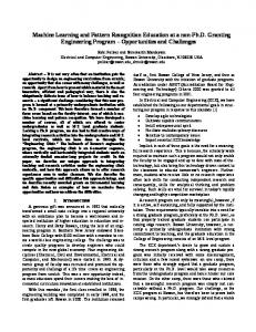
𝐻𝑖𝑑𝑑𝑒𝑛 𝑙𝑎𝑦𝑒𝑟𝑠: # 𝑟𝑜𝑤𝑠 < # 𝑟𝑜𝑤𝑠 + # 𝑟𝑜𝑤𝑠 < 2 ∗ 3 # 𝑟𝑜𝑤𝑠. (14) Fig 2: Neural network structure for software project The input defines the input attributes that are cost drivers of past and present project and actual software cost. The output
When the Neural Net is trained with hidden layers in the range (14) the accuracy is improved and NN is trained with low training error.
14
International Journal of Computer Applications (0975 – 8887) Volume 89 – No 16, March 2014
5.2 Fuzzy logic trained NN (FLNN)
5.4 Naïve Bayes Classifier (NBC) Table 3.Naive Bayes Confusion Matrix
Pred. range 1 Pred. range 2 Class recall
Fig 3: FLNN graph showing mapping of FIS output on training data The training data is the actual cost and the FIS output is the predicted cost using fuzzy logic. The close mapping of values shows that NN is better trained using Fuzzy logic. The RMSE error of FLNN is 0.136 which shows much improvement over Decision Tree, Naïve Bayes and Perceptron. . A membership function µ(X) describes the membership of the elements x of the base set X in the fuzzy set A. A membership function is defined for those sets of data where precise classification is not possible; hence membership domain is defined based on cluster centers [6]. The “index” on the x axis is the Epoch rate to train the neural network. The membership function graph is Gaussian type depicting 4 cluster centers (2 for each input attribute) generated from the software project dataset
5.3 Decision Tree
True range 1 7
True range 2 4
Class precision 63.54
1
1
50.00
87.50
20.00
Naïve bayes classifier classifies the information based on Bayesian probability as shown in figure 6. A Bayesian probability is considered to be an evidential probability in which evidences that is cost drivers and actual software cost data is analyzed to predict the cost. The Bayesian theorem is an extension of propositional logic (true/false) that enable to reason uncertainty which exists in S/W cost [8]. In naïve bayes classifier, hypothesis is created which is renewed in the light of new, relevant data. The true range defined in the table is the actual value. The prediction range is defined as (Pred. Range 1)Negative (∞,0.500] and (Pred. range 2) Positive (∞, 0.500]. A recall of 20% defines lower rate of irrelevant instances. Accuracy of the result achieved is 62%.
5.5 Linear Regression (LR) Linear regression is another machine learning technique used in SCE. The RMSE for linear regression shows much improvement than NN, naïve bayes classifier, FLNN. The linear regression uses the concept of curve fitting using linear equation intercept form. LR technique finds its application in forecasting, prediction. Given a variable y and a number of variables X1, X2, X3….Xn that may be related to y LR technique can be applied to deduce the relationship between Xi and y. This relationship is shown in terms of weights. P values