Learning from History for Behavior-Based Mobile Robots in Non

Machine Learning, 31, 141–167 (1998)

c 1998 Kluwer Academic Publishers, Boston. Manufactured in The Netherlands. °

Learning from History for Behavior-Based Mobile Robots in Non-Stationary Conditions FRANCOIS ¸ MICHAUD

[email protected]

Department of Electrical and Computer Engineering, Université de Sherbrooke, Sherbrooke, Québec, Canada J1K 2R1 [email protected] Computer Science Department, University of Southern California, Los Angeles, CA 90089-0781

´ MAJA J. MATARIC

Editors: Henry Hexmoor and Maja J. Matarić Abstract. Learning in the mobile robot domain is a very challenging task, especially in non-stationary conditions. The behavior-based approach has proven to be useful in making mobile robots work in real-world situations. Since the behaviors are responsible for managing the interactions between the robots and its environment, observing their use can be exploited to model these interactions. In our approach, the robot is initially given a set of “behaviorproducing” modules to choose from, and the algorithm provides a memory-based approach to dynamically adapt the selection of these behaviors according to the history of their use. The approach is validated using a vision- and sonar-based Pioneer I robot in non-stationary conditions, in the context of a multi-robot foraging task. Results show the effectiveness of the approach in taking advantage of any regularities experienced in the world, leading to fast and adaptable specialization for the learning robot. Keywords: multi-robot learning, history-based learning, non-stationary conditions, self-evaluation

1.

Introduction

Learning in the mobile robot domain requires coping with a number of challenges, starting with difficulties intrinsic to the robot. These difficulties are caused by incomplete, noisy, and imprecise perception and action, and by limited processing and memory capabilities. These affect the robot’s ability to represent the environment and to evaluate the events that take place. Increasing the perceptual and computational abilities of the robot is possible to some extent, but is accompanied by a larger state space and consequently an increase in learning time and in the complexity of the system. Furthermore, stationary conditions (or slowlyvarying non-stationary conditions) are typically required to enable a robot to learn a stable controller or a model of the environment. However, in dynamic environments such as the multi-robot domain, the dynamics are particularly important, making the learning task even more difficult. Finally, a general conclusion from the robotics and control applications is that it has proven necessary to supplement the fundamental learning algorithm with additional pre-programmed knowledge in order to make a real system work (Kaelbling et al., 1996, Mahadevan & Kaelbling, 1996). This method bypasses complete autonomy by giving up tabula rasa learning techniques (Kaelbling et al., 1996) in favor of incorporating bias that accelerates the learning process and then allowing to further refine and alter that initial policy over time, as the dynamics change. This implies that learning must take place while underlying situations and conditions (like obstacle avoidance, navigation, tasks) are being managed in real-time.

142

´ F. MICHAUD AND M.J. MATARIC

Behavior-based systems (Brooks, 1986, Maes, 1989, Matarić, 1992b) have been praised for their robustness and simplicity of construction. They have been shown to be effective in various domains of mobile robot control, allowing the systems to adapt to the dynamics of real-world environments. Such systems are commonly composed of a collection of “behavior-producing” modules that map environment states into low-level actions, and a gating mechanism that decides, based on the state of the environment, which behavior’s action should be switched through and executed (Kaelbling et al., 1996). Many robot learning algorithms use this methodology, mostly by learning to associate percepts with actions to learn a behavior (Floreano & Mondada, 1996, del R. Millán, 1996, Mahadevan & Connell, 1992), or to associate percepts with behaviors (Matarić, 1994b, Matarić, 1997), or both (Dorigo & Colombetti, 1994, Asada et al., 1994). The objective in using behaviors is to try to minimize the learner’s state space, and maximize learning at each trial (Matarić, 1994a). Initial knowledge for a learning robot can take the form of a set of behaviors, defining its skills for handling the situations encountered in its environment and for accomplishing its goals. Learning is then localized at the gating mechanism. To the extent to which they can be anticipated, initial associations between percepts and behaviors can also be programmed in. However, many real-world tasks involve partial observability, i.e., the state of the environment is incompletely known from the current, immediate percepts (McCallum, 1996a, McCallum, 1996c). One interesting solution to this problem is to use history, i.e., to explicitly take into consideration the time sequence of observations. History information can be learned form percepts and actions (McCallum, 1996b), but for large or continuous spaces it also requires extensive training periods. Considering history at the behavior level would allow reduction of the learning space, and would be based on the use of the controlling resources (i.e., the behaviors) responsible for managing the robot’s interactions with its operating environment. The learned model could then be used to change the way the robot responds to the perceived conditions. This is especially useful in the case of unpredictable and non-stationary environments (as in the multi-robot domain) where the world’s dynamics are difficult for the designer to characterize and to fully predict a priori, and would thus be best captured by the robot itself. Using this idea, we propose a learning algorithm that allows the robot to monitor its interactions with its operating environment so as to alter its behavior selection. The robot is initially given a set of behaviors, whose subset is used to accomplish the assigned tasks safely. The goal of the algorithm is to learn to select alternative behaviors that are not normally exploited, to adapt the robot’s behavior to the experienced dynamics. The selection is based on a tree representation of history and on a performance criterion, both derived from the observation of past behavior use. The history of behavior use allows this memorybased algorithm to learn a model of typical interactions, i.e., repeatable dynamics. We demonstrate and validate our approach on a vision- and sonar-based Pioneer I robot in the context of foraging in a multi-robot environment. To present the details of the proposed algorithm and the obtained results, this paper is organized as follows. Section 2 gives a detailed explanation of the learning algorithm. Section 3 describes the experimental setup and the mobile robots used in the experiments, and Section 4 presents the experimental results. A discussion concerning the properties

LEARNING FROM HISTORY

143

of the learning algorithm is given in Section 5. Section 6 summarizes related work, and Section 7 concludes the paper. 2.

History-based learning for adaptive behavior selection

Within the behavior-based framework, a robot needs different types of “behavior-producing” modules to operate in its environment. These behaviors can be classified according to their respective purposes. In our approach, this classification is useful for analyzing the interactions derived from observing behavior use. Behaviors for achieving specific operations (e.g., search-for-object, go-to-place, pick-up, drop) are required by the robot to accomplish its tasks. Other behaviors are required for safe navigation in the environment (e.g., avoid-obstacles). We call the first type “task-behaviors”, and the second “maintenancebehaviors”. Both types are triggered in response to specific conditions in the environment, which can be pre-programmed. The robot can also use behaviors that introduce variety into its action repertoire (like wall-following, small-turn, rest, etc.). We call these “alternativebehaviors”. In contrast to the other types of behaviors, no a priori conditions are given to activate alternative-behaviors. The algorithm we describe learns to activate these behaviors according to the robot’s past experiences. Note that a behavior can be activated (i.e., selected), but may not have direct control of the robot; the actual control of the robot’s effectors is based on the behavior’s rules that generate actions and on the overall subsumption organization of the control system (Brooks, 1986) (see Section 3). In general, a behavior is considered to be “in use” only when it controls the actions of the robot. Our approach is composed of four parts: 1) a tree-based mechanism for representing the sequences of behavior use; 2) an evaluation metric; 3) a recommendation mechanism for selecting alternative-behaviors, and 4) a path deletion mechanism. We describe each in turn. 2.1.

The tree representation mechanism

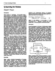
As the robot tries to accomplish one of its tasks, behaviors are executed and their sequence is stored within a tree structure representing the history of their use. The nodes of the tree store two items: the name or the type (for task-behaviors) of the behavior (both represented by a letter, e.g., A for the Avoidance) being executed, and the number of times a transition between the node itself and its successor has been made, as shown in Figure 1. For synchronization reasons, the root node of a tree is always a task-behavior node, i.e., whatever behavior is used at the start of the task. Initially, the tree for a particular task is empty and is incrementally constructed as the robot goes about its task. Leaf nodes are characterized by the letter E (for end-node) and store the total performance of the particular tree path. Whenever a path is completely reused, i.e., when the same sequence of behaviors is executed, the average of the stored and current performances for the last 10 trials (this number was determined empirically from various experiments) is computed and stored in E (Figure 1 also shows the tree in list notation later used in Section 4). The history of behavior use and the resulting performance values give the robot the ability to learn to trigger alternativebehaviors according to the observed dynamics.

144


S,5

A,5

S,3

A,3

S,3

E,3

60%

F,2

A,2

S,1

E,1

80%

T,1

S,1

E,1

70%

((S 5) (A 5) ((S 3) (A 3) (S 3) (E 3 60)) ((F 2) (A 2) ((S 1) (E 1 80)) ((T 1) (S 1) (E 1 70))))

Figure 1. Tree representation of the history of behavior use, followed by its list notation. For clarity, junctions are indented so the sub-paths are aligned.

2.2.

Metric for self-evaluation of performance

Performance can be evaluated using a variety of factors. Given a robot with limited capabilities operating in a dynamic environment, optimality is difficult to define and may also be non-stationary. As a possible solution to this problem, we explored time of behavior use as the key evaluation metric. However, other metrics could be used in different domains and for different tasks. Our evaluation function, expressed by Relation 1 below, is characterized by the amount of time required to accomplish the task and the interference experienced during that process: ¶¶ µ µ (t − T T ) (ttb − tmb + tc ) (1) − max 0, eval(t) = max 0, ttb TT where tb refers to task-behaviors, mb to maintenance-behaviors, and t to the current time-step (corresponding to one cycle of evaluation of all currently active behaviors). The first term of Relation 1 reflects the amount of control the robot has over the task, expressed as the relationship between task-behavior and maintenance-behavior uses. Without considering tc , this term is positive when task-behaviors are used more than maintenancebehaviors; otherwise it is negative. Since the evaluation function is bounded between 0 and 100%, if tmb becomes much larger than ttb , it would take an equivalent period of time before eval(t) becomes greater than 0. Since the purpose of this evaluation function is to discriminate between the experienced situations, we added tc , a correction factor that increases when eval(t) decreases below 0%. It enables eval(t) to increase as soon as a task-behavior is used, allowing better discrimination between trials. Note that the variation of eval(t) monotonically decreases as the duration of task-behavior use increases, which helps characterize the interactions experienced in the environment. The second term of Relation 1 penalizes the robot’s performance if it takes more time to accomplish the task than it has in the past. T T represents the average total number of time-steps taken to accomplish the task over the last 10 trials, updated upon completion of a task. Again, the number 10 was determined empirically by analyzing typical results; it

145


establishes a compromise between adaptability to changes in the environment and tolerance for poor performance resulting from necessary exploration of different options. T T captures changes in the dynamics of the environment that affect the time to complete the task. 2.3.

Recommendation criteria for selecting alternative-behaviors

In addition to being used at end-nodes, eval(t) is also evaluated at time t to decide whether or not an alternative-behavior should be tried. More precisely, the algorithm has different options: not to make any changes in its active behavior set (this option is referred as the Observe option), or to recommend the activation of an alternative-behavior. Different selection criteria can be used by comparing the performance at the current position in the tree (i.e., eval(t)) with the expected performance. The expected performance of a given node is the sum of the stored end-node performances in its sub-paths, multiplied by the frequency of use of the sub-paths relative to the current position in the tree. Formally, the expected performance for sub-path i starting from a given position in the tree is given by Relation 2: X nj eval(T )j · (2) Ei (eval) = ni j where j refers to the end-nodes accessible from sub-path i, eval(T )j is the performance memorized in these end-nodes, and n is the number of times the node j of sub-path i was visited. This gives the expected performance for each sub-path in a tree, i.e., for each possible option at the current position in the tree. To get the expected performance at this position, a similar formula is used, as expressed by Relation 3: E(eval) =

X i

Ei (eval) ·

ni n

(3)

A simple example of the application of these formulas can be given using the bold node in Figure 1 as the current node. The expected performance of the S sub-path is 60·3/3 = 60%, while the expected performance of the F sub-path is (80·1/2)+(70·1/2) = 75%. The total expected performance E(eval) for this node would then be (60 · 3/5) + (75 · 2/5) = 66%. Note that longer paths do not necessarily mean lower performance; the evaluation function is not influenced by the number of different nodes in the path but by the time spent during behavior use. Using the expected performances at the current position in the tree and those at each of its sub-paths, the choice made by the algorithm is based on the following criteria: •

If (eval (t) ≥ E(eval)), then take the option with the maximum expected performance Ei (eval). This criterion is referred as the TM criterion, for Try Maximum. If only one sub-path exists at the current position in the tree, then the best option from the nearest junction following this sub-path is taken, but only if all of the options have already been tried. This allows the robot to explore the options sooner, and limits the depth of the tree while still being biased toward using the best option.

•

If (eval (t) < E(eval)), then two possible situations exist:

146


–

If there are untried options at this junction, then select an untried option. This selection criterion is referred to as UO, for Untried Option. If multiple untried options exist, one is chosen randomly.

–

If there are no untried options at this junction, choose the one with overall best performance (i.e., over all the trials up to that point). The overall best option is obtained from a Global Options Table (GOT), an array of past performances indexed by the name of the option. The GOT is updated at the end of each trial by averaging the resulting performance with the ones stored, for all the options used for that trial. Since in this case the tree does not provide a choice of options, the GOT enables the algorithm to chose the option that showed the best global performance in the past. The GOT mechanism also prevents consecutive recommendation of the same option during a trial, and shows preference to untried options in order to encourage uniform exploration and avoid “local maxima” in the early stages of learning.

To summarize, the choice made by the algorithm is based on three criteria (TM, UO, and GOT), as follows: 1. IF (eval (t) ≥ E(eval)) THEN 2. Take sub-path with max(Ei (eval)) (TM criterion) 3. ELSE IF there are untried options at this junction THEN 4. Select Untried Option (UO criterion) 5. ELSE Select the option with overall best performance from the Global Options Table (GOT criterion) The evaluation of the recommendation criteria takes place only at a maintenance-behavior node (i.e., node created by the observation of a maintenance-behavior) because that is when interference occurs in the accomplishment of the robot’s tasks, resulting in decreased eval(t). When one of these nodes is reached, the recommendation can be directly set by UO or GOT if eval(t) is already lower than E(eval), or by TM if eval(t) is greater or equal to E(eval). If this condition changes at the given position in the tree, UO or GOT can override the selection made using TM. Note also that when a new path is constructed, its expected performance is 0 and the default option is to behave without using any alternativebehaviors. This allows the robot to explore what can be accomplished by using task- and maintenance-behaviors only. 2.4.

Path deletion mechanism

Since this algorithm is used in noisy and non-stationary conditions, deleting paths is necessary to keep the interaction model that the tree represents up to date. More specifically, because the expected performance is a weighted average based on the frequency of occurrences of the sub-paths, the most tried option at a given maintenance-node will have a greater influence on E(eval). This decreases the variation of E(eval) as an option is tried frequently, making it harder to modify it and to change strategies if the option becomes in fact less useful. In those conditions, forgetting may be as important as learning (Albus, 1991).


147

Forgetting paths may lead to exploring some of the choices again and discovering changes in the world. Node deletion also serves to regulate memory use. To enable the robot to respond to recent changes in the environment, we opted for deleting the oldest path in the tree when more than d different paths were stored. The trial number stored in the end-nodes determined the oldest path; when it is deleted, the n values of the nodes in the tree are updated accordingly. Other criteria can be easily substituted for different applications. 3.

Experimental setup and task description

Our experiments were performed on a Real World Interface Pioneer I mobile robot (shown on the right of Figure 2) equipped with seven sonars and a Fast Track Vision System. The robot is programmed using MARS (Multiple Agency Reactivity System) (Brooks, 1996), a Lisp-based language for programming multiple concurrent processes and behaviors. The robot on the left in Figure 2 is an IS Robotics R1 robot used in the multirobot experiments, equipped with infra-red and contact sensors. The experiments were conducted in an enclosed 12’×11’ rectangular pen which contains pink blocks and a home region, indicated with a green cylinder. These colored objects were perceived using the robot’s vision system. Other obstacles and walls were detected using the sonar system; the dark stripe on the wall of the pen is a strip of corrugated cardboard used to improve sonar reflection. The R1 robots were perceived as obstacles by the Pioneer’s sonars. The behavior of the Pioneer robot was also influenced by: •

Limitations of the vision system. The robots’ vision system is noisy, has a limited field of view, and suffers from variations in light intensity at different places in the pen and from different angles of approach. This made the robot miss blocks up to 20% of the time, and miss the home region less than 10% of the time. Because our Pioneer robots did not have grippers, nor could use vision to see their own front end, we had to use an internal state variable to maintain the presence or absence of the block in front of the robot and this too was affected by the imprecision of the vision system. Additionally, noise is not evenly distributed over different trials and different sensors.

•

Limitations of control. The actions of the robot were sometimes influenced by the presence of debris on the floor and by general effector noise.

•

Limitations of processing and computational resources. On the Pioneer robot, the delay between sensing and acting is 0.2 seconds. Since the robot is continuously moving, this results in different turning rates near an obstacle and an imprecise dropping point at home. In addition, garbage collection freezes the commands sent to the robot for 1 second, making it possible to hit an object or to miss a target during that period.

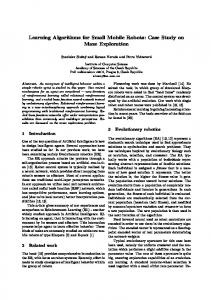
The overall subsumption (Brooks, 1986) organization of the behaviors used in our experiments is shown in Figure 3. The behaviors control the velocity and the rotation of the robot based on sonar readings and visual inputs. The robot is given two tasks: search for a block (“Searching Task”), and bring it to the home region (“Homing Task”). Separate learning trees are used for each task, determined by the activated task-behavior. In our experiments, the robot had one specific task-behavior for the Searching Task, called Searching-block, and

148


Figure 2. A Pioneer I robot (on the right) near a block, the home region, and an R1 robot.

two for the Homing Task, Homing and Drop-block. A task-behavior called Velocity-control was activated in both of these tasks to make the robot move. Conditions for activating task-behaviors were pre-programmed based on the presence or absence of a block in front of the robot, and the proximity to home. The Searching-block behavior was activated when no block was being pushed by the robot and 10 seconds after dropping a block at home. The Homing behavior was activated when a block was being pushed, and the Drop-block behavior was activated when the robot got close enough to the home region. The Avoidance behavior was used for handling harmful situations and interference (detected using the sonars) while the robot was accomplishing its task. This behavior was normally activated except near home when the robot was carrying a block, allowing close approach of the home region. When used, the Avoidance behavior subsumes task-behaviors and takes over the control of the robot. Finally, the alternative-behaviors available were Follow-side, Rest and Turn-randomly. When selected, alternative-behaviors were activated for pre-set periods of time determined by the designer: five seconds for Rest, and ten seconds for Follow-side and Turn-randomly. Note that these behaviors are not designed to be mutually exclusive: functionality can emerge by activating many behaviors at the same time, especially given the overall subsumption organization of the system. For example, Follow-size and Homing can issue commands consecutively, creating the emerging functionality of going home by following a wall. Initial bias is also present in the subsuming organization of the behaviors: Follow-side is allowed to subsume Homing and Searching-block in order not to go straight to the goal, but instead to change the way of reaching it (e.g., by following the wall). However, Turn-randomly is, by design, not allowed to subsume these task-behaviors because its purpose is to help the robot see its target, and not turn away from it. Whenever a behavior is executed, the symbol associated with it (e.g., F for Follow-side, R for Rest, etc.) is added (by still following the subsuming organization of behaviors) to the symbol sequence representing the behavior use at each processing cycle. The sequence is used to construct and update the interaction model, i.e., the tree. The node type (S for the Searching Task and H for the Homing Task) is used to identify the use of a task-behavior in the tree, while the actual symbol of maintenance and alternative-behaviors are used to

149


Recommendation of alternative-behavior Tree representation of history of behavior use Behavior sequence VVVAAAAAAAASSSSSSSSSVVVTTTVVVAAAA...

Interaction Model Level Behavior Level R A D F S H T V

Rest Avoidance Drop-block Follow-side Searching-block Homing Turn-randomly Actions Velocity-control

Figure 3. Overall organization of the behaviors and the model learned from observing behavior use. Activated behaviors for the Searching Task, with Turn-randomly as a chosen alternative-behavior, are depicted in bold.

discriminate different situations in the interactions experienced by the learning robot. At each time step, the current symbol is processed to determine the position in the tree (by following nodes in the tree or by creating a new one). The timing counters ttb , tmb and tc are also incremented accordingly. If the current node is a maintenance-node, the expected performance is evaluated and recommendation of alternative-behaviors is done according to the criteria presented in Section 2.3. Finally, when the task is completed or a task change occurs, T T is updated and the performance is stored in the current end-node of the tree and in the GOT for that task. The path deletion mechanism is also used when appropriate. Learning is done over several trials of the robot accomplishing its tasks. 4.

Experiments

Although the goal of the proposed algorithm is to learn in dynamic environments, it would have been inappropriate to start directly with a multi-robot domain experiment where nonstationary conditions make the analysis and the validation of the properties of the algorithm extremely difficult. To gradually address this problem, we first used static environment conditions with increasing complexity to verify that the algorithm could learn stationary conditions from its interactions with the environment. Next, experiments with multiple robots were performed. The same behavior repertoire was used in both sets of experiments, without optimization or retraining of the vision system parameters for color detection. The objective was to create situations where the designer could not know or adjust the behaviors according to a priori knowledge of the environment. All the computations were done on-board with a limited amount of memory (the entire robot program used 66 Kbytes of

150


memory, with 27 Kbytes used by the learning algorithm, leaving 43 Kbytes for storing the trees; a tree of 200 nodes takes approximately 7 Kbytes). To evaluate the performance of the learning algorithm, we collected traces of all choices made, E(eval) at the first junction of the trees, T T , eval(T ), and the number of nodes added and deleted in each trial. The analysis of this data, collected in the different environment configurations, is presented in the following subsections: Section 4.1 presents the results obtained with static environment conditions, showing the properties of the components of the learning algorithm; Section 4.2 describes the results of the group experiments and the usefulness of the algorithm in making the robot learn in dynamic environment conditions. We describe only the results obtained for the Searching Task because they best illustrate the properties of the learning algorithm. A complete description of all of the experimental results can be found in (Michaud & Matarić, 1997). 4.1.

Static environment conditions

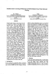
Three different environmental configurations were used for the experiments in static conditions. The first one used three blocks at the corners of the pen, with the home region in the fourth corner. In this setup, the Pioneer was able to see the block from almost everywhere in the environment, and had to find its way back to the home region. Five experiments of 60 to 115 trials were done, each lasting between 1.5 and 2 hours, using this simple configuration. The main purpose was to validate the algorithm. Although the learned strategies did not involve complex use of alternative-behaviors (since the goals of finding a block or finding home were easily perceivable in the pen), the results showed that the algorithm could learn to use alternative-behaviors only when they were needed. Specifically, the robot learned, based on the trees and eval(t), that alternative-behaviors were useful after missing a block or the home region. The second environmental configuration used one block in the center of the pen, as shown in Figure 4. To find the block, the Pioneer had to move away from the boundaries of the pen in order to see the block in the center. Twenty-two experiments of 40 to 120 trials were done, each lasting from 1 to 3 hours and validating different properties of the algorithm. Finally, the third configuration used boxes to divide the pen into two regions, and placed the block in the region opposite from home, thus increasing the level of difficulty in finding it. This configuration is shown in Figure 6. Eleven experiments of approximately 45 trials were done, lasting 2 hours each. Figure 5 shows the different behavior strategies that were learned by the robot for the configuration with the block in the center. In this configuration, not using any alternativebehavior did not result in a good solution: the robot could loop around the block for some time before being able to see it. The learned strategies involved using Follow-side and Rest. After dropping the block at home using the Drop-block behavior, the robot usually started to search for a block from the 1st corner or the 3rd corner. As represented by the dotted line, using the Follow-side behavior from the 1st corner made the robot follow the wall to the 2nd corner, where it could see the block and easily bring it to the home region. From the 3rd corner, using the same option made the robot either follow the wall to the 2nd corner, or go directly for the block (when it was visible from the corner) by trying to follow the wall (strategy “F and S” in Figure 5). This resulted in an interesting emergent functionality. In addition, Rest was found to be useful for doing this task. Using Rest in front of a wall

151


Figure 4. Environmental configuration with one block placed in the center of the pen.

3rd corner

2nd corner F and S

F

TR

R 1st corner

Figure 5. Behavior selection strategies learned for the Searching Task in the configuration with one block placed in the center of the pen.

made the robot rotate more than when Avoidance was exploited right away, helping it see the block directly from that location. This interesting dynamic was not anticipated and resulted in a strategy efficient in both the 1st and 3rd corners of the pen. The robot also learned to use other options if Rest alone was not successful in finding the block. Finally, we were surprised to find that Turn-randomly was not frequently useful. Because this behavior makes the robot rotate by a random angle at a random interval, it is not very reliable in helping the robot see the block. In fact, it frequently made the robot loop around the block. It is important to note that all of these discoveries were made by the robot from its own point of view, instead of by the designer. With the pen divided into two regions, not using any alternative-behaviors made the robot usually go to the 3rd corner. From this corner the robot was able to see the block until it hit the obstacle in the middle of the pen, making it turn away and loose the block from its field of view. It then turned most of the time toward the 2nd corner. This trajectory

152


Figure 6. Environmental configuration with the pen divided into two regions.

F and S

TR

Figure 7. Behavior selection strategies learned for the Searching Task with the pen divided into two regions.

is depicted with the dotted line in Figure 7. A different Searching-block behavior with a short-term memory of the location of the block before turning away could have prevented this. However, we did not anticipate this situation during the design, and did not want to change the behavior repertoire during the experiments. As stated earlier, the goal was to see how the robot could manage without optimization of its behaviors by the designer. This was particularly important for scaling up to the multi-robot experiment where various kind of interference could happen when searching for a block, and where such special-purpose fixes would not have been possible. The strategies learned by the robot to accomplish the Searching Task involved mostly Turn-randomly, Rest and Follow-side. The robot learned not to go into the 3rd corner (by using Turn-randomly) or if there, to use an alternativebehavior like Follow-side to avoid having to move toward the boxes and lose the block. Finally, another interesting and unanticipated strategy was Rest – Rest, i.e., use Rest in front of the first and second obstacle encountered by the robot (illustrated in Figure 8). Because of the particular dynamic created by using this behavior in front of a static obstacle (as

153


explained previously), this usually resulted in avoiding the 3rd corner and allowing the robot to easily pick up the block.

R R

Figure 8. Rest – Rest strategy learned for the Searching Task with the pen divided into two regions.

Using the list notation introduced in Figure 1, Figure 9 shows a tree learned by the robot after 60 trials with the block in the center configuration. E(eval)i values for the sub-paths at the first junction in the tree are also shown. At the first junction in this tree, the Observe option (marked with ‘***’) is the one with maximum E(eval)i , followed by Follow-side. Note that this path may or may not be followed depending on eval(t) and the use of the selected option. As it turned out for this example, the option Observe is recommended, but usually eval(t) became lower than E(eval) and then the GOT recommended the use of the Follow-side behavior. The performance in the GOT for the tree of Figure 9 is presented in Table 1. Had the learning continued, the Observe path would probably have been deleted since it was the third oldest path stored in the tree: Follow-side would than have become the preferred path. The Observe option worked well at the beginning of the experiment, and then became difficult to reproduce. Recommending the Follow-side behavior using the GOT started after the 24 trials and was used frequently (37 times out of the 50 trials stored in the tree), resulting in a stable strategy. A stable strategy is recognized by having a predominant sub-path as deep as possible in the tree, surrounded by sub-paths for the other options to ensure that the preferred options of the predominant sub-path are still valid. This can also be corroborated by Figure 10, showing the stabilization of the number of nodes in the tree, indicating that the paths in the tree adequately represent the interactions experienced by the robot in its environment. Finally, we can see that there were two possibilities after Followside was observed: a task-behavior can be used (Case 1), which happened most of the time, or a maintenance-behavior was used (Case 2). This made it possible to discriminate between two different situations based on the behaviors used, so that distinct strategies were learned to handle these cases appropriately. The results obtained using these environmental configurations show that the different components of the learning algorithm try to establish a compromise between exploration (learning to adapt to noise and changes in the environment) and exploitation (Kaelbling et al., 1996) of a stable behavior selection strategy. The evaluation function

154


Figure 9. Searching Task tree after 60 trials for an experiment using the configuration with the block in the center.

characterizes the current situation and the past experiences. The tree representation captures sequences of behavior use in a compact fashion to make a decision based on past experiences. The recommendation criteria exploit both of these components to determine when and what choice to make. They manage the exploration/exploitation process of this learning algorithm: the TM criterion favors exploitation of the options, while the UO and GOT criteria favor exploration for the purpose of finding a different best option. Finally, path deletion influences the choices made by affecting E(eval) in the tree.

155


Number of nodes in the tree - Searching Task 250

Number of nodes

200

150

100

50

0 0

10

20

30 Trial number

40

50

60

Figure 10. Graph of the number of nodes in the tree for the Searching Task of an experiment using the configuration with the block in the center. Table 1. Performance values stored in the GOT for the tree shown in Figure 9. Alternative-behavior Observe Follow-side Turn-randomly Rest

evalGOT (%)

Number of behavior use

32 56 24 26

8 40 9 13

Analysis of the results also revealed three important properties of the learning algorithm: •

The GOT plays an intermediate role between exploration of options at a given node (when the algorithm does not know which choice to make), and exploitation of the option with the best performance. It serves as a medium-term memory of the performances of the options. Having a stable strategy using the TM criterion reinforces the GOT option part of this strategy. This prevents a valid strategy from being modified by small perturbations affecting the experienced performance. At the same time, the GOT makes the learning algorithm adapt more easily to changes in the environment that can be reflected in a more constant fashion in the performance of the trials. For a frequently used strategy, E(eval) is more difficult to change because its evaluation is made according to a larger number of trials. In contrast, the GOT is not subject to this and allows for faster exploration by exploiting outcomes of recent trials. The GOT criterion is preferred to random behavior selection because it favors using knowledge derived from past experiences instead of blindly exploring all of the options.

•

Establishing a compromise between exploration and exploitation is affected by the deletion factor d. Increasing this factor helps create strategies with longer sequences

156


of nodes. However, having a small deletion factor does not prevent learning longer strategies; it only requires a greater number of consecutive, stable and reproducible events in the environment. The deletion factor defines the storage capability of the algorithm, which can also be viewed as a principled bias set up by the designer. More precisely, we believe that this factor should be set according to the number of different nodes in the tree and the kind of adaptability the designer wants the robot to manifest. It also helps to look at the number of trials required to find a stable strategy or to see the stabilization of E(eval), but this is not necessary and the learning algorithm will adapt to this choice. In our experiments, setting this parameter to 25 showed to be sufficient in rapidly generating long strategies and allowing fast adaptation to changes. •

4.2.

An initial strategy can serve as a bias toward the elaboration of a specialized way of behaving, but does not prevent it from changing dynamically. To validate this point, we performed some experiments by starting with the configuration with one block in the center, and then changing it to the one dividing the pen into two regions. Figures 11 and 12 show the plot of E(eval) at the first junction of the tree and the number of nodes in the tree for the learning trials of one of this experiment. The first 60 trials were done with the block in the center configuration, which resulted in learning a stable strategy of using the Follow-side behavior. Then, a two-phase change occurred: the strategy changed to using the Observe option for a while, and then Rest from trial 87 on. This can be seen from the changes in E(eval). In fact, Observe and Rest were the second and third best options at the first junction of tree before the change of configuration occurred. The change of strategies and the stabilization starting around the 87th trial is also corroborated by Figure 12, demonstrating that the algorithm was able to quickly adapt to changes in the environment. In effect, the approach shows transfer of what was learned in the first configuration to what was useful in the new, second configuration.

Dynamic environment conditions using multiple robots

For the multi-robot experiments, the block to be brought home was put in the center of the pen, as shown in Figure 13. Two or three R1 robots were added to the scenario, and generated interference in the environment. The R1s were programmed to move about, avoid all obstacles and stay out of forbidden regions using their contact and infra-red sensors, mounted in the front and below their grippers. These forbidden regions were the areas of the pen that were marked with dark tiles or tape, i.e., the area surrounding the block, the home region, and one dark-tiled corner of the pen. The R1 controller was simple: when detecting an obstacle or a forbidden area, the robots moved backward and turned away from the obstacle, then moved forward again; otherwise, they moved forward freely. These constraints on the R1s’ motion resulted in a great deal of dynamic interference. Additionally, although dark areas were inaccessible to the R1s, sensor noise enabled them to occasionally enter those areas nonetheless. Using this configuration, fifteen experiments of 60 to 80 trials were run, lasting between 1.5 and 2 hours and using two or three R1s. In some of these experiments, two learning Pioneer robots were used to compare their learned strategies. However, when placed together, additional sources of noise affected the behaviors of the robots: 1) when facing

157


E(eval) at the first junction - Searching Task 100 90 80 70

%

60 50 40 30 20 10 0 30

40

50

60 70 Trial number

80

90

100

Figure 11. Graph of E(eval) for the Searching Task tree of an experiment starting with the configuration with one block in the center, and then changing to the configuration dividing the pen into two regions. Number of nodes in the tree - Searching Task 550 500 450

Number of nodes

400 350 300 250 200 150 100 30

40

50

60 70 Trial number

80

90

100

Figure 12. Graph of the number of nodes for the Searching Task tree of an experiment starting with the configuration with one block in the center, and then changing the configuration dividing the pen into two regions.

each other at particular angles, crosstalk between the sonars sometimes occurred; 2) one Pioneer robot searching for a block could perceive and pursue the block pushed by the other; 3) the blue Pioneer robot sometimes confused the red Pioneer robot with a pink block. During these experiments, the non-stationary conditions arose from the presence and movement of the R1s, and varied greatly during and between the experiments. In some cases, one or two R1s stayed close to the home region, while in others all moved around

158


Figure 13. Environmental configuration for the multi-robot experiments, with two Pioneers and three R1s. The R1s are programmed to avoid obstacles and the areas marked with dark tiles or tape.

the region near the block. As the learning is primarily dependent on the sequence of past experiences, which changes in each experiment run, optimality cannot be determined from the task alone (unless a very large amount of data is available for statistical analysis). To counter this, we used the run-time data and studied the experiment video tapes in order to analyze what, why, and how strategies were learned, if regularities were found from the interactions dynamics, and how the algorithm adapted to changes detected from these interactions. For the Searching Task, the learned strategies largely involved the use of Observe, Rest and Turn-randomly. The sequences of options learned were: Observe – Rest; Observe – Rest – Observe; Rest; Rest – Turn-randomly; Rest – Observe; and Turn-randomly. The strategies changed over time according to past experiences. One or two stable strategies “won out” in most runs. Figure 14 shows a tree learned by the robot after 68 trials, and Table 2 presents the performance stored in the corresponding GOT. Table 2. Performance values stored in the GOT for the Searching Task tree in a multi-robot experiment. Alternative-behavior Observe Follow-side Turn-randomly Rest

evalGOT (%)

Number of behavior use

34 20 24 19

41 26 14 29

Figure 15 shows the trace of the choices made for the first and the last 20 trials of the same experiments. Data associated with a choice are delimited by parentheses and consist of the trial number, the name of the option chosen, the name of the selection criterion used, eval(t) and E(eval) at the position of the tree where the choice was made. In the initial trials, Follow-side was the first favored option. However, this strategy did not remain stable for long; from trials 28 to the end of the experiment, the Observe – Rest strategy was


159

Figure 14. Searching Task tree for a multi-robot experiment.

preferred (e.g., in trials 48–50, 58, 62, 63, 65–68). Between these trials, different options were explored. These choices were made using the TM and GOT criteria. Consecutive choices with the same E(eval) values indicate that they were made from the same position in the tree. Notice that for trials 49, 50, 51, 53, 62, 64 and 66, a choice using the TM criterion is overridden by one made using the UO or the GOT criterion because eval(t) fell below E(eval). Shorter paths are a sign that the robot was able to find the block without experiencing much interference from the R1s. Otherwise, longer sequences of choices were

160


Figure 15. Trace of choices made for the Searching Task tree in a multi-robot experiment.

generated because longer paths were reused. Finally, Figure 16 shows that the number of nodes stopped increasing and started to decrease around the 50th trial, demonstrating reuse of stored paths in the tree, even in non-stationary conditions. From Figure 14, it is also possible to see that the algorithm allowed the robot to discriminate two situations using the Observe – Rest strategy: using Rest in front of a static obstacle (Case 1) and using Rest in front of a moving obstacle (Case 2). This distinction is made according to the behavior used after resting, without using any special processing to

161


Number of nodes in the tree - Searching Task 350

300

Number of nodes

250

200

150

100

50

0 0

10

20

30 40 Trial number

50

60

70

Figure 16. Graph of the number of nodes in a Searching Task tree in a multi-robot experiment.

distinguish a moving from a static obstacle, and lead to distinct strategies for behavior selection. This revealed to be a very interesting property of the learning algorithm. Additional observations made from these experiments are: •

When two Pioneer robots are put in the pen at the same time, they can specialize differently in their ways of accomplishing the task. In one experiment, strategies learned by one Pioneer for the Searching Task were Observe – Rest – Observe and Rest – Turn-randomly, while the other learned to mostly use Turn-randomly. For the Homing Task, Follow-side – Turn-randomly was learned by one robot, while Rest was used by the other. Additionally, the Searching Task for one Pioneer revealed more complex interactions than for the other: one tree had 468 nodes compared to 256 for the other. Thus, although both robots were in the “same” environment conditions, they specialized toward different strategies based on their specific, individual experiences. Having two Pioneers or more R1s in the pen did not influence the Pioneers’ ability to find stable strategies; the dynamics of the interaction with the environment had a more significant effect.

•

We mentioned earlier that many strategies were used interchangingly by the robots: when performance for one strategy decreased, another one was used based on what was learned previously. For example, suppose that the preferred strategy is Rest and the second best strategy learned in the past is Turn-randomly – Rest. If the second best strategy becomes the preferred one, paths memorized for this option are used again. This phenomenon happened frequently in our experiments and allowed the elaboration of longer strategies and of parallel “solutions.” It depended on finding a stable set of possible strategies and keeping a sufficient number of paths in the tree. Conversely, having to go deeper in the tree makes it more difficult to completely reuse paths.

162 5.


Discussion

The fundamental idea behind the presented algorithm is that the performance of situated or embedded systems is based on their ability to cope with and to exploit the dynamics of interactions with their environment (Agre, 1988, Brooks, 1991). Since we decided to use behaviors for controlling the robot, it was most appropriate to model these interactions using a representation mechanism consistent with the behavior-based framework. Doing so also preserves two key strengths of the behavior-based approach, situatedness and emergence (Brooks, 1991), but also adds a cognitive aspect to the system, allowing it to model its interactions. In our approach, behaviors can be considered to be implicit short-term models of the world, simultaneously capturing the different factors involved in the decision process. Behaviors serve as building blocks, more abstract than percepts and actions, for constructing a representation of the experienced interactions and for evaluating the robot’s experience. The tree representation is used to situate the robot relative to those interactions, and create a context in which to evaluate similar situations. The evaluation function used in our experiments differs from commonly used approaches that typically attempt to optimize external criteria such as time required to accomplish the task, total distance traveled, number of collisions, etc. The performance of a robot situated in a dynamic environment and having an incomplete view of the world is difficult to evaluate using traditional, externally-measured criteria. This is the case at least in part because typical evaluation criteria were developed for and adapted from very different, more static and predictable domains. In the case of robots using a decentralized and distributed framework without explicit communication, it becomes difficult to design an optimization formula that would efficiently represent all possible situations. When communication between robots is used, different group policies or arbitration schemes can be pre-programmed (Goldberg & Matarić, 1997, Fontán & Matarić, 1996, Matarić, 1994a), but the question of knowing which policy to apply according to different factors (like group size and group density) remains. Another reason for not using such of an approach is that special care would have had to be taken during the design of alternative-behaviors so that their use would have a similar impact on the optimization criteria. However, using behaviors as an abstraction for evaluating performance sacrifices some precision granted by an optimization function that can correctly represent what needs to be learned, but ensures faster learning and does not constrain what can be learned by the robot. Non-stationary conditions make it difficult to evaluate learning performance, and in that case we try to show that optimality may not be formally determined from the task, but rather from the specific experiences of the robot. Consequently, there may exist many efficient strategies for the given task, and the approach aims for reasonably efficient behavior in accordance with the robot’s abilities to interact with the environment. In those conditions, it may be more appropriate to evaluate learning performance by the ability of the approach to make consistent decisions based on past experiences, with a good balance between exploration and exploitation of the options. The results demonstrate that the algorithm has this ability. Using the non-monotonic decreasing performance function of Relation 1 enabled “selfevaluation” by the learning algorithm. This makes the learning independent of the constraints of the environment, the tasks, the limitations of the robot and the specifics of the designed behaviors. For example, alternative-behaviors were subsuming different groups


163

of behaviors, and each was learned to be used by the robot in specific situations. It also helped generate unanticipated behavior selection strategies, decreasing the burden of behavior design by not having to fine-tune the behaviors or acquire knowledge about the specific and complex dynamics of the system. For example, a slightly different angle of the camera changed the field of view of the robot, and although we tried to keep it constant it was not possible to guarantee that it was placed at the same position in all experiments. Fortunately, our approach does not depend on such levels of precision and calibration but only requires that behaviors be designed to help establish distinctions between different interaction dynamics and derive an effective representation. This allows the robot to learn strategies that are difficult and unlikely for the designer to anticipate. In effect, these influences allow the algorithm to establish critical points for behavior selection, i.e., decision factors for recommending the activation of behaviors. These critical points are self-determined and modified in response to continuing changes in the dynamics, which could be caused by alterations of the environment, the behavior of other robots, or the variability of the robot’s abilities (e.g., due to noise, battery power, etc.). Even in a nonstationary environment, these critical points provide the robot with some ability to make expectations based on previous experiences, and thus evaluate its current performance. As indicated in Section 2.2, any kind of optimization function can be used as the evaluation function for our learning algorithm. In the context of our experiments, the evaluation function we used proved to be adequate in making the robot learn useful information quickly to control its behavior in stationary and non-stationary conditions. Overall, it did not require the robot to have special perceptual or computational abilities: instead, the learning algorithm made the robot do the best it could with what it had. Criteria based on behavior use, like the frequency of use of behaviors, could have been useful and will be studied in future experiments. Another possible extension is to associate percepts and action to links between nodes to get a more precise discrimination between options to take at a junction in the tree, or couple the approach with another knowledge representation formalism to encode information about the world. Using percepts and actions versus behaviors are two different ways of representing knowledge about the world, but they are not mutually exclusive and can co-exist within a system. Their combination is likely to be explored in future work. 6.

Related work

The described robot learning approach is related to methodologies from the field of machine learning, principally with the reinforcement learning paradigm. Reinforcement learning is defined as the problem faced by an agent that learns behavior through trial-and-error interactions with a dynamic environment, without needing to specify how the task is to be achieved (Kaelbling et al., 1996). Our work deals with three important issues in reinforcement learning: incomplete and imperfect perception, learning by using prior knowledge, and multi-agent learning (Mahadevan & Kaelbling, 1996). In our approach, the decision is derived from stored past experiences and the current situation in the tree; an action takes the form of a behavior recommendation, and the reward is based on the internal measure of performance, which is also deduced from behavior use over time. A key difference from the commonly used reinforcement learning algorithms is that we did not use a scalar

164


reinforcement signal, or one completely determined by perceived conditions. In addition, as with other learning approaches, learning time depends on the size of the learning space, i.e., the number of different options to select from. In our experiments, both tasks used the same set of alternative-behaviors, but subsets of alternative-behaviors can be specified to limit the search for distinct tasks. Previous approaches to learning behavior selection (Maes & Brooks, 1990, Mahadevan & Connell, 1992, Matarić, 1997) used sensory inputs as the selection criterion. In contrast, our approach introduces the use of the stored history within the behavior-based framework, making it possible to learn regularities in the robot’s interactions with its environment which are difficult to pre-program. This approach in a compromise between model-free behaviorbased reinforcement learning (e.g., for behavior selection) and full model-based work. A related approach, learning from observed behavior activation (but not behavior use), was explored in the case-based reasoning framework in work by (Ram & Santamaria, 1993). The approach learns a behavior activation strategy based on history over a time window from inputs and from past behavior activation. A case-based algorithm is used to retrieve similar cases, adapt the activation of behaviors, and learn new associations or adapt existing cases. A reward signal is used to maximize consistency in “useful” behaviors, and a robot simulator is used to validate the approach. The computational complexity of this approach is much greater than ours. An approach to using behaviors as the underlying representation for constructing a model within a behavior-based system was done by (Matarić, 1992a). In this work, the navigating mobile robot associated landmarks in the environment with specific behaviors, and connected those behaviors into a network whose topology was isomorphic to the explored environment. The behaviors stored the landmark type (similar to our node-type) and compass direction, and spread activation to dynamically direct the robot toward a goal landmark, in a simple form of behavior selection. Representing history information using a tree representation was inspired by the work of (McCallum, 1996b, McCallum, 1996c), concerned with learning for agents with physical and computational restrictions. His approach partitions the state space from raw sensory experiences, and uses memory of features to augment the agent’s perceptual inputs. This way, history information allows the representation to be interpreted in the context of the flawed state space (McCallum, 1996a), i.e., to bias this representation according to perceptual constraints. The raw-experience-representing “instances” are encoded in a U-tree, starting from the root node and following the branches labeled by a feature that matches its observations. These features have a perceptual dimension (sensory data or actions) and a history index (time step backward). The leaves of the tree store utility estimates (Q-values) that are used to choose the next action. This mechanism is successfully applied to learning to drive in a virtual highway environment. Globally, the U-Tree approach learns a variable-width window that serves simultaneously as a model of the environment and a finite-memory policy (Kaelbling et al., 1996). Comparatively, our algorithm learns a finite-memory strategy of behaviors use and selection, since it uses behaviors as an abstraction. In addition to applying a different performance measure, our approach differs from McCallum’s in the selection criteria. While the U-Tree algorithm follows the path with maximum expected reward and random exploration, our algorithm compares the current with the expected performance from the tree and the GOT. Additionally, exploration is also


165

affected by the path deletion mechanism, while the U-Tree uses statistic evaluation at the leaf nodes. Our approach is very different from dynamic programming approaches which aim at finding a probability-based state/action table for maximizing utility values. In our case, behaviors serve as an abstraction for both state (behavior use) and action (behavior selection), and the decision process does not optimize a fixed utility function. Instead, our algorithm tries to capture and characterize the experienced dynamics based on the tree representation and the evaluation function. This results in continuous adaptation of what is being “optimized” in the behavior of the robot, without requiring extensive training periods to model changes in non-stationary conditions. Finally, the development of our algorithm was derived from a general control architecture for an intelligent agent (Michaud et al., 1996) based on dynamic selection of behaviors. The notion of observation of behavior use, called Behavior Exploitation, is used to make the system monitor the proper satisfaction of its “intentions”, as expressed by the selected behaviors. The approach described in the current paper demonstrates that observing behavior use can also be a rich source of information for learning a representation of the robot’s interactions with its operating environment and for evaluating its performance, information that can be useful for behavior selection (Michaud, 1997). 7.

Conclusion

Learning in dynamic and unpredictable environments, as in the multi-robot domain, is a very challenging problem. The goal of our approach is to enable a robot to learn and utilize the interaction dynamics with its environment from self-evaluation of its behavior. The learning algorithm uses history of behavior use to derive an incrementally-updated tree representation as a model of these interactions. Learning the model and using it to derive behavior selection strategies are done relative to the exploitation of the controlling resources (i.e., the behaviors) of the robot. In that regard, the algorithm is oriented toward continuous life-time adaptation rather than on learning a one-time, static policy. The approach is computationally efficient and demonstrated on-board two mobile robots in real-time and in dynamic and noisy conditions. Results show that the approach allows a consistent selection of behaviors according to the conditions prevailing in the environment and the robot’s past experiences. They demonstrate the effectiveness of the approach in taking advantage of any regularities experienced in the world, leading to fast and adaptable robot specialization. Furthermore, they indicate that to get an efficient robot learning algorithm for dynamic and non-stationary conditions, it might be preferable not to attempt to learn a globally optimal behavior choice (which relies on perceptual limitations and long learning trials). The interaction with the environment is affected by the dynamics and the robot’s own limitations in perception, action and processing, but none of those are typically precisely characterizable a priori. Instead, our approach advocates internal evaluation of the interaction dynamics, and taking advantage of them while they are still valid. By doing so, the approach leads to learning unanticipated behavior strategies from the perspective of the robot instead of the designer, thus increasing robot autonomy. Overall, the proposed approach can be compared to learning idiosyncratic and specialized ways of behaving in complex environments. It also provides a predictive

166


capability that is typically lacking in behavior-based systems, thus making a move toward increasingly “cognitive” means for generating complex behavior. Acknowledgments Support for the Postdoctoral Fellowship of Fran¸cois Michaud was provided by NSERC (Natural Sciences and Engineering Research Council of Canada). This research is also funded by the Office of Naval Research Grant N00014-95-1-0759 and the National Science Foundation Infrastructure Grant CDA-9512448 to Maja J. Matarić. The authors thank Prem Melville for his help during the experiments, Barry Werger for his patience and assistance in debugging and programming of the robots, and Dani Goldberg, Miguel Schneider Fontán and the rest of the Interaction Lab for their insightful comments. References Agre, P. E. (1988). The Dynamic Structure of Everyday Life. PhD thesis, Massachusetts Institute of Technology, Cambridge, MA. Albus, J. S. (1991). Outline for a theory of intelligence. IEEE Trans. on Systems, Man, and Cybernetics, 21(3):473–509. Asada, M., Uchibe, E., Noda, S., Tawaratsumida, S. & Hosoda, K. (1994). Coordination of multiple behaviors acquired by a vision-based reinforcement learning, Proc. IEEE/RSJ/GI Int’l Conf. on Intelligent Robots and Systems, Munich, Germany. Brooks, R. A. (1986). A robust layered control system for a mobile robot. IEEE Journal of Robotics and Automation, RA-2(1):14–23. Brooks, R. A. (1991). Intelligence without representation. Artificial Intelligence, 47:139–159. Brooks, R. A. (1996). MARS: Multiple Agency Reactivity System (Technical Report IS Robotics). Cambridge, MA. del R. Millán, J. (1996). Rapid, safe, and incremental learning of navigation strategies. IEEE Trans. on Systems, Man, and Cybernetics—Part B: Cybernetics, 26(3):408–420. Dorigo, M. & Colombetti, M. (1994). Robot shaping: Developing autonomous agents through learning. Artificial Intelligence, 71(4):321–370. Floreano, D. & Mondada, F. (1996). Evolution of homing navigation in a real mobile robot. IEEE Trans. on Systems, Man, and Cybernetics—Part B: Cybernetics, 26(3):396–407. Fontán, M. S. & Matarić, M. J. (1996). A study of territoriality: the role of critical mass in adaptive task division. In P. Maes, M. J. Matarić, J.-A. Meyer, J. Pollack & S. Wilson, editors, From Animals to Animats: Proc. 4th Int’l Conf. on Simulation of Adaptive Behavior, Cape Cod: The MIT Press. Goldberg, D. & Matarić, M. J. (1997). Interference as a tool for designing and evaluating multi-robot controllers. Proc. National Conf. on Artificial Intelligence (AAAI) (pp. 637–642), Providence, RI. Kaelbling, L. P., Littman, M. L. & Moore, A. W. (1996). Reinforcement learning: A survey. Journal of Artificial Intelligence Research, 4:237–285. Maes, P. (1989). The dynamics of action selection. Proc. Int’l Joint Conf. on Artificial Intelligence (IJCAI) (pp. 991–997), Detroit, MI. Maes, P. & Brooks, R. A. (1990). Learning to coordinate behaviors. Proc. Nat’l Conf. on Artificial Intelligence (AAAI), Vol. 2 (pp. 796–802). Mahadevan, S. & Connell, J. (1992). Automatic programming of behavior-based robots using reinforcement learning. Artificial Intelligence, 55:311–365. Mahadevan, S. & Kaelbling, L. P. (1996). The NSF workshop on reinforcement learning: Summary and observations. AI Magazine. Matarić, M. J. (1992a). Integration of representation into goal-driven behavior-based robots. IEEE Transactions on Robotics and Automation, 8(3):46–54. Matarić, M. J. (1992b). Behavior-based systems: Key properties and implications. Proc. IEEE Int’l Conf. on Robotics and Automation, Workshop on Architectures for Intelligent Control Systems (pp. 46–54), Nice, France.


167

Matarić, M. J. (1994a). Interaction and intelligent behavior (MIT AI Lab AI-TR 1495). Massachusetts Institute of Technology, Cambridge, MA. Matarić, M. J. (1994b). Reward functions for accelerated learning. In W. W. Cohen & H. Hirsh, editors, Proc. 11th Int’l Conf. on Machine Learning (pp. 181–189), New Brunswick, NJ: Morgan Kauffman Publishers. Matarić, M. J. (1997). Reinforcement learning in the multi-robot domain. Autonomous Robots, 4(1). McCallum, A. K. (1996a). Hidden state and reinforcement learning with instance-based state identification. IEEE Trans. on Systems, Man, and Cybernetics—Part B: Cybernetics, 26(3):464–473. McCallum, A. K. (1996b). Learning to use selective attention and short-term memory in sequential tasks. In P. Maes, M. J. Matarić, J.-A. Meyer, J. Pollack & S. W. Wilson, editors, From Animals to Animats: Proc. 4th Int’l Conf. on Simulation of Adaptive Behavior (pp. 315–324), Cape Cod: The MIT Press. McCallum, A. K. (1996c). Reinforcement learning with selective perception and hidden state. PhD thesis, Department of Computer Science, University of Rochester, USA. Michaud, F. (1996). Nouvelle architecture unifiée de contrôle intelligent par sélection intentionnelle de comportements. PhD thesis, Department of Electrical and Computer Engineering, Université de Sherbrooke, Québec, Canada. Michaud, F. (1997). Adaptability by behavior selection and observation for mobile robots. In R. Roy, P. Chawdry and P. Pants, editors, Soft Computing in Engineering Design and Manufacturing. Springer-Verlag. Michaud, F. & Matarić, M. J. (1997). A history-based learning approach for adaptive robot behavior selection (Technical Report CS-97-192). Computer Science Department, Volen Center for Complex System, Brandeis University, Waltham, MA, USA. Michaud, F., Lachiver, G. & Dinh, C. T. L. (1996). A new control architecture combining reactivity, deliberation and motivation for situated autonomous agent. In P. Maes, M. J. Matarić, J.-A. Meyer, J. Pollack & S. W. Wilson, editors, From Animals to Animats: Proc. 4th Int’l Conf. on Simulation of Adaptive Behavior (pp. 245–254), Cape Cod: The MIT Press. Ram, A. & Santamaria, J. C. (1993). Multistrategy learning in reactive control systems for autonomous robotic navigation. Informatica, 17(4):347–369. Received September 1, 1997 Accepted December 30, 1997 Final Manuscript February 1, 1998