Oct 2, 2017 - corresponding Hamiltonian is free from the sign problem [NU98; GKW16; Suz93]. Third, Tensor. 1. arXiv:1710.00725v1 [quant-ph] 2 Oct 2017 ...
Learning hard quantum distributions with variational autoencoders Andrea Rocchetto1,2 , Edward Grant1 , Sergii Strelchuk3 , Giuseppe Carleo4 , and Simone Severini1,5
arXiv:1710.00725v1 [quant-ph] 2 Oct 2017
1
Department of Computer Science, University College London 2 Department of Materials, University of Oxford 3 DAMTP, University of Cambridge 4 Institute for Theoretical Physics, ETH Zurich 5 Institute of Natural Sciences, Shanghai Jiao Tong University
Abstract Studying general quantum many-body systems is one of the major challenges in modern physics because it requires an amount of computational resources that scales exponentially with the size of the system. Simulating the evolution of a state, or even storing its description, rapidly becomes intractable for exact classical algorithms. Recently, machine learning techniques, in the form of restricted Boltzmann machines, have been proposed as a way to efficiently represent certain quantum states with applications in state tomography and ground state estimation. Here, we introduce a new representation of states based on variational autoencoders. Variational autoencoders are a type of generative model in the form of a neural network. We probe the power of this representation by encoding probability distributions associated with states from different classes. Our simulations show that deep networks give a better representation for states that are hard to sample from, while providing no benefit for random states. This suggests that the probability distributions associated to hard quantum states might have a compositional structure that can be exploited by layered neural networks. Specifically, we consider the learnability of a class of quantum states introduced by Fefferman and Umans. Such states are provably hard to sample for classical computers, but not for quantum ones, under plausible computational complexity assumptions. The good level of compression achieved for hard states suggests these methods can be suitable for characterising states of the size expected in first generation quantum hardware.
1
Introduction
A known challenge in the numerical analysis of quantum systems is the exponential growth of the number of parameters required to describe a system, as a function of its size. From numerically integrating Schroedinger’s equation to quantum state tomography, the size of the system is a key limiting factor in the use of exact methods. The numerical simulation of interacting quantum systems then mainly relies on techniques which handle the exponential complexity of the wave function in special cases, and use different inspiring principles. First, exact diagonalisation methods, which rely on the exact representation of the many-body state [LP04; NM05; JB08; L¨ au11], and thus are limited to small systems. Second, quantum Monte Carlo methods (QMC), that allow one to efficiently sample from ground and finite-temperature states, provided the corresponding Hamiltonian is free from the sign problem [NU98; GKW16; Suz93]. Third, Tensor
1
Network approaches (TN), relying instead on low-entangled representations of quantum states, that are especially effective for one-dimensional lattice systems [VMC08; Or´ u14]. Recently, machine learning methods have been introduced to tackle a variety of tasks in quantum information processing that involve the manipulation of quantum states. These techniques offer greater flexibility and, potentially, better performance, with respect to the methods traditionally used. Research efforts have focused on representing quantum states in terms of restricted Boltzmann machines (RBMs). Those are physically-inspired generative models, with a single layer of hidden neurons, that allow one to approximate high-dimensional functions, as well to efficiently generate samples from them. The main advantage of using RBMs is that certain quantities, like marginals, can be estimated analytically. Furthermore, they can be used to learn unknown probability distributions, using unsupervised machine learning techniques. This representation of the wave function, introduced by Carleo and Troyer [CT17], has been successfully applied to reconstruct quantum states from experimental measurements – the goal of quantum state tomography – by Torlai et al. [Tor+17]. While for compressing many-body states RBMs have shown good performance in practice, theoretical analysis of their functioning has only been established for their multilayer variant – Deep Boltzmann Machines (DBMs) – where strong representability results have been shown. In particular, Gao and Duan [GD17] proved that two-layer DBMs with complex-valued weights can efficiently represent most physical states. Although this result is of great theoretical interest, the practical application of complex-valued DBMs in the context of unsupervised learning has still not been demonstrated. Three major questions then still remain to be addressed. First, deep networks have been shown to achieve better performance with respect to shallow ones in almost every practical ML task. Does the same apply to quantum states? How does the depth of the network influence our ability to compress a state? Second, the performance of shallow RBMs has been benchmarked on types of states that are known to be tractable with classical computers (e.g., matrix product states (MPS) [Per+06]). How do these methods perform on states that are known to be hard to learn (or even to approximate)? Third, is it possible to devise a practical numerical scheme to take advantage of deep architectures? In this paper, we address these problems, and introduce a method for representing the probability distribution defined by a quantum state based on variational autoencoders (VAEs) [KW13]. VAEs are state of the art in many generative problems, i.e. problems where a learner seeks to generate samples from an unknown probability distribution based on a training set. We investigate two aspects of this representation: we discuss how the depth of the network affects the network’s ability to compress quantum many-body states; we determine the extent to which hard quantum states can be compressed. The first question has been previously addressed by Metha and Schwab [MS14] and Gao and Duan [GD17]. However, these works do not discuss how depth affects the capability of a network of representing states of different complexity. Here, we specifically focus on understanding the role played by depth in representing states of different hardness. This question is particularly important if one seeks to determine whether neural network models can efficiently capture quantum features. Indeed, classical results [MLP16; Tel16; ES16] show that depth significantly improves the representational capability of networks for some classes of functions (such as compositional functions). Our numerical simulations show that depth consistently improves the quality of the reconstruction for hard states that can be efficiently constructed with a quantum computer. The same does not apply for hard states that cannot be efficiently constructed by means of a quantum process. Here, depth does not improve the reconstruction accuracy. This empirical observation might signal that some types of neural network are able to detect correlations that are specific to quantum states. 2
The second question has important implications in the verification and characterisation of quantum systems. Beyond certain size thresholds which are about to be exceeded by existing quantum computers, simulation of their properties becomes classically intractable, and there is a growing demand for techniques that will be able to verify various properties of such devices. The VAE representation provides one such technique – it can assist in the verification of small quantum computers by reducing the number of parameters required to represent their computational states. Although it can be proved that in order to construct an approximate description of a general quantum state, a procedure also known as quantum state tomography, one must perform exponentially (in the number of qubits) many measurements [OW16] our simulations indicate that, for states with a number of qubits that is likely to be implemented on first generation quantum hardware, the VAE representation can provide a reduction in the number of parameters up to a factor 5. This improvement might make VAE states a promising tool for the characterisation of early quantum devices that are expected to have a number of qubits that is slightly larger than what can be efficiently simulated using existing methods [Boi+16]. This paper is structured as follows. Section 2 introduces the VAEs representation of quantum states. Testing the efficacy of this representation on states of different hardness is one of the key contributions of this work. We discuss the complexity theoretic framework on the learnability of quantum states and how to generate hard states in Section 3. The next two sections analyse the performance of the VAE representation. In Section 4, we present numerical experiments showing that deeper networks perform better when learning hard quantum states. In light of this result, we propose the VAE representation as a useful tool to probe near future quantum hardware. This is discussed in Section 5, where we present numerical simulations showing that the number of parameters required to learn an n-qubit hard quantum state can be significantly reduced. Conclusions are in Section 6.
2
Encoding quantum probability distributions with VAEs
Variational autoencoders (VAEs), introduced by Kingma and Welling in 2013 [KW13], are generative models based on layered neural networks. Given a set of i.i.d. data points X = {x(i) }, where x(i) ∈ Rn , generated from some distribution pθ (x(i) |z) over Gaussian distributed latent variables z and model parameters θ, finding the posterior density pθ (z|x(i) ) is often intractable. VAEs allow for approximating the true posterior distribution, with a tractable approximate model qφ (z|x(i) ), with parameters φ, and provide an efficient procedure to sample efficiently from pθ (x(i) |z). The procedure does not employ Monte Carlo methods. As shown in Fig. 1 a VAE is composed of three main components. The encoder that is used to project the input in the latent space and the decoder that is used to reconstruct the input from the latent representation. Once the network is trained the encoder can be dropped and, by generating samples in the latent space, it is possible to sample according to the original distribution. In graph theoretic terms, the graph representing a network with a given number of layers is a blow up of a directed path on the same number of vertices. Such a graph is obtained by replacing each vertex of the path with an independent set of arbitrary but fixed size. The independent sets are then connected to form complete bipartite graphs. The model is trained by minimising over θ and φ the cost function: J(θ, φ, x(i) ) = −Ez∼qφ (z|x(i) ) [log pθ (x(i) |z)] + DKL (qφ (z|x(i) )||pθ (z))).
(1)
The first term (reconstruction loss) −Ez∼qφ (z|x(i) ) [log pθ (x(i) |z)] is the expected negative loglikelihood of the i-th data-point and favours choices of θ and φ that lead to more faithful reconstructions of the input. The second term (regularisation loss) DKL (qφ (z|x(i) )||pθ (z))) is the 3
Figure 1: Encoding quantum probability distributions with VAEs. A VAE can be used to encode and then generate samples according to the probability distribution of a quantum state. Each dot corresponds to a neuron and neurons are arranged in layers. Input (top), latent, and output (bottom) layers contain n neurons. The number of neurons in the other layers is a function of the compression and the depth. Layers are fully connected with each other with no intra layer connectivity. The network has three main components: the encoder (blue neurons), the latent space (green), and the decoder (red). Each edge of the network is labelled by a weight θ. The total number of weights m in the decoder corresponds to the number of parameters used to represent a quantum state. The network can approximate quantum states using m < 2n parameters. The model is trained using a dataset consisting of basis elements drawn according to the probability distribution of a quantum state. Elements of the basis are presented to the input layer on top of the encoder and, during the training phase, the weights of the network are optimised in order to reconstruct the same basis element in the output layer. Kullback-Leibler divergence between the encoder’s distribution qφ (z|x(i) ) and the Gaussian prior on z. A full treatment and derivations of the variational objective are given in [KW13]. VAEs can be used to encode the probability distribution associated to a quantum state. Let us consider an n-qubit quantum state |ψi, with respect to a basis {|bi i}i=1,...,2n . We can write the probability distribution corresponding to |ψi as p(bi ) = |hbi |ψi|2 . If we consider the P n computational basis, we can write |ψi = 2i=1 ψi |ii, where each basis element corresponds to an n-bit string. A VAE can be trained to generate basis elements |ii according to the probability p(i) = |hi|ψi|2 = |ψi |2 . We note that, in principle, it is possible to encode a full quantum state (phase included) in a VAE. This requires samples taken from more than one basis and a network structure that can distinguish among the different inputs. The development of VAE encodings for full quantum states will be left to future work. We approximate the true posterior distribution across measurement outcomes in the latent space z with a multivariate Gaussian, having diagonal covariance structure, zero mean and unit standard deviation. The training set consists of a set of basis elements generated according to the distribution associated with a quantum state. Following training, the variables z are sampled from a the multivariate Gaussian and used as the input to the decoder. By taking samples from this Gaussian as input, the decoder is able to generate strings corresponding to measurement outcomes that closely follow the distribution of measurement outcomes used to train the network. 4
3
Generating hard and easy quantum states
As discussed in the introduction, the description of a general quantum state requires a number of parameters that grows exponentially with the system size. However, there exist special families of non-trivial quantum states (e.g. stabiliser states [AG04] or states with vanishing entanglement) for which one can produce a description that uses only linear number of parameters. We thus want to test neural network models which may efficiently represent quantum states which have varying complexity of representation. For example, for states that admit an efficient representation, can networks learn this representation? Similarly, for quantum states which encode probability distributions which are conjectured to be hard to sample from on a classical computer, how does the accuracy of representation scale with the depth of a network? The common theme of these questions is whether neural networks are able to efficiently capture the correlations present in quantum states. Here we introduce the conceptual framework for answering these questions. We consider different types of quantum states whose representational complexity, as well as computational effort required for their generation, ranges from polynomial to exponential. To date, a complete classification of states with an efficient representation is still beyond reach. Many physical states have efficient representations (e.g. MPS) but so do many states with prominent quantum features (e.g. Greenberger-Horne-Zeilinger (GHZ) states [GHZ89]). The problem of determining which states have an efficient representation appears to be related to the problem of finding efficiently learnable states. A framework to analyse the learnability of quantum states has been proposed by Aaronson [Aar07]. Here, all quantum states are shown to be probably approximately correct (PAC)-learnable from an information-theoretic perspective. The problem of which class of quantum state is also efficiently learnable (i.e. learnable with a polynomial amount of computational resources) remains open. The only class of states that is known to be efficiently PAC-learnable [Roc17] also admits an efficient representation. For our purposes, we define easy to be such states which have an efficient classical description (such as stabiliser states or MPS with low bond dimension). These states can be expressed using a number of parameters which scale proportionally to the log of the dimension. We distinguish two types of hard states: 1) states that can be efficiently constructed with a quantum computer, but are conjectured to have no classical algorithm to do so; 2) states that cannot be efficiently obtained on a quantum computer starting from some fixed product input state (e.g. random states). In the next section we test the VAE representation on all three kind of states. Specifically, for the class of easy states we consider separable states obtained by taking the tensor product of N n different 1-qubit random states. More formally, we consider states of the form |τ i = ni=1 |ri i where |ri i are random 1-qubit states. These states can be described using only 2n parameters. Among the class of hard states of the first kind, we study the learnability of a class of hard distributions introduced in [Fef14] which can be sampled exactly on a quantum computer. These distributions are conjectured to be hard to approximately sample from classically – the existence of an efficient sampler would lead to the collapse of the Polynomial Hierarchy under some natural conjectures described in [Fef14; AA11]. We discuss how to generate these kind of states in Appendix B. Finally, for the second class of hard states, we consider random pure states. These are generated by normalising a 2n dimensional complex vector drawn from the unit sphere according to the Haar measure.
5
4
The role of depth in compressibility
Classically, depth is known to play a significant role in the representational capability of a neural network. Recent results, such as the ones by Mhaskar, Liao, and Poggio [MLP16], Telgarsky [Tel16], and Eldan and Shamir [ES16] showed that some classes of functions can be approximated by deep networks with the same accuracy as shallow networks but with exponentially less parameters. The representational capability of networks that represent quantum states remains largely unexplored. Some of the known results are only based on empirical evidence and sometimes yield to unexpected results. For example, Morningstar and Melko [MM17] showed that shallow networks are more efficient than deep ones when learning the energy distribution of a 2dimensional Ising model. In the context of the learnability of quantum states Gao and Duan [GD17] proved that DBMs can efficiently represent some states that cannot be efficiently represent by shallow networks (i.e. states generated by polynomial depth circuits or k-local Hamiltonians with polynomial size gap). However, there are no known methods to sample efficiently from DBMs when the weights include complex-valued coefficients. We benchmark with numerical simulations the role played by depth in compressing states of different levels of complexities. We focus on three different states: an easy state (the completely separable state discussed in Section 3), a hard state (according to Fefferman and Umans), and a random pure state. Our results are presented in Fig. 2. Here, by keeping the number of parameters in the decoder constant, we determine the reconstruction accuracy of networks with increasing depth. Remarkably, depth affects the reconstruction accuracy of hard quantum states. This might indicate that VAEs are able to capture correlations in hard quantum states. As a sanity check we notice that the network can learn correlations in random product states and that depth does not affect the learnability of random states. Our simulations suggest a further link between neural network and quantum states. This topic has recently received the attention of the community. Specifically, Levine et al. [Lev+17] demonstrated that convolutional rectifier networks with product pooling can be described as tensor networks. By making use graph theoretic tools they showed that nodes in different layers model correlations across different scales and that adding more nodes to deeper layers of a network can make it better at representing non-local correlations.
5
Efficient compression of physical states
In this section we focus our attention onto two questions: can VAEs find efficient representations of easy states? What level of compression can we obtain for hard states? Through numerical simulations we show that VAEs can learn to efficiently represent some easy states (that are challenging for standard methods) and achieve good levels of compressions for hard states. Remarkably, our methods allow to compress up to a factor 5 the hard quantum states introduced in [FU15]. We remark that the exponential hardness cannot be overcome for general quantum states and our methods achieve only a factor improvement on the overall complexity. This may nevertheless be sufficient to be used as a characterisation tool where full classical simulation is not feasible. We test the performance of the VAE representation on two classes of states: the hard states that can be constructed efficiently with a quantum computer introduced by Fefferman and Umans [FU15] and states that can be generated with a long-range Hamiltonian dynamics, as found for example in experiments with ultra-cold ions [Ric+14]. The states generated through this 6
0.928 0.9925 0.938 0.9900
F
F
F
0.926
0.936
0.924
0.9875
0.922
0.934
0.9850 1
2
3
4 L
5
(a)
6
7
1
2
3
4
1
2
3
L
(b)
4 L
5
6
7
(c)
Figure 2: Depth affects the learnability of hard quantum states. Fidelity as a function of the number of layers in the VAE decoder for (a) an 18-qubit hard state that is easy to generate with a quantum computer, (b) random 18-qubit product states that admit efficient classical descriptions and (c) random 15-qubit pure states. Errors bars for (b) and (c) show the standard deviation for an average of 5 different random states. The compression level C is set to C = 0.5 for (a) and (c) and C = 0.015 for (b) where C is defined by 2mn where m is the number of parameters in the VAE decoder and n is the number of qubits. We use a lower compression rate for product states because, due to their simple structure, even a 1 layer network achieves almost perfect overalp. Plot (b) makes use of up to 4 layers in order to avoid the saturation effects discussed in Appendix A. evolution are highly symmetric physical states. However, due to the bond dimension increasing exponentially with the evolution time, these states are particularly challenging for MPS methods. An interesting question is to understand whether neural networks are able to exploit these symmetries and represent these states efficiently. We describe long-range Hamiltonian dynamics in Appendix C. Results are displayed in Fig. 3. For states obtained through Hamiltonian evolution we achieve with almost maximum reconstruction accuracy compression levels of up to C ' 10−3 . This corresponds to a number of parameters m = O(100) � 218 which implies that the VAE has learned an efficient representation of the state. In the case of hard state we can reach a compression level of 0.2, corresponding to a compression factor of 5 . Similar levels of compression could play a role in experiments aimed at showing quantum supremacy. In this setting a quantum machine with a handful of noisy qubits performs a task that is not reproducible even by the fastest supercomputer. As recently highlighted by Montanaro and Harrow [HM17] one of the key challenges with quantum supremacy experiments is to verify that the quantum machine is behaving as expected. Because quantum computers are conjectured to not be efficiently simulatable, verifying that a quantum machine is performing as expected is a hard problem for classical machines. The review by Gheorghiu, Kapourniotis, and Kashefi [GKK17] provides an introduction to several approaches to verification of quantum computation. Our methods might allow to characterise the result of a computation by reducing the complexity of the problem.
6
Conclusions
In this work we introduced VAEs, a type of deep, generative, neural network, as way to encode the probability distribution of quantum states. Our methods are completely unsupervised, i.e. 7
0.932
1.0
0.930 0.928
0.6 F
F
0.8
0.926
0.4 0.924 0.2 0.0
0.922 0.5e-3 1.0e-3 1.5e-3 2.0e-3 2.5e-3 3.0e-3 C
0.2
(a)
0.3
0.4 C
0.5
0.6
(b)
Figure 3: VAEs can learn efficient representation of easy states and can be used to characterise hard states. Fidelity as a function of compression C = m/2n for (a) an P 18-qubit state generated by evolving 2−n/2 i |ii using the long-range Hamiltonian time evolution described in Appendix C for a time t = 20 and (b) an 18-qubit hard state generated according to [FU15]. Figure (a) shows that the VAE can learn to represent efficiently with almost perfect accuracy easy states that are challenging for MPS. Figure (b) shows that hard quantum states can be compressed with high reconstruction accuracy up to a factor 5. The decoder in (a) has 1 hidden layer to allow for greater compression without incurring in the saturation effects discussed in Appendix A. The decoder in (b) has 6 hidden layers in order to maximise the representational capability of the network. do not require a labelled training set. By means of numerical simulations we showed that deep networks can represent hard quantum states that can be efficiently obtained by a quantum computer better than shallow ones. On the other hand, for states that are hard and conjectured to be not efficiently producible by quantum computers, depth does not appear to play a role in increasing the reconstruction accuracy. Our results suggest that neural networks are able to capture correlations in states that are provably hard to sample from for classical computers but not for quantum ones. As already pointed out in other works, this might signal that states that can be produced efficiently by a quantum computer have a structure that is well represented by a layered neural network. Through numerical experiments we showed that our methods have two important features. First, they are capable of representing using fewer parameters states that that are known to have efficient representation but where standard methods like MPS struggle. Second, VAEs can compress hard quantum states up to a constant factor. However low, this compression level might enable to approximately verify quantum states of a size expected on near future quantum computers. Presently, our methods allow to encode only the probability distribution of a quantum state. Future research should focus on developing VAE architectures that allow to reconstruct the full set of amplitudes. Other interesting directions involve finding methods to compute the quantum evolution of the parameters of the network and investigating whether the depth of a quantum circuit is related to the optimal depth of a VAE learning its output states. Finally, it is interesting to investigate how information is encoded in the latent layers of the network. Such analysis might provide novel tools to understand the information theoretic properties of a
8
quantum system.
Acknowledgements Andrea Rocchetto and Edward Grant contributed equally to this work. We thank Carlo Ciliberto, Danial Dervovic, Alessandro Davide Ialongo, Joshua Lockhart, and Gillian Marshall for helpful comments and discussions. Andrea Rocchetto is supported by an EPSRC DTP Scholarship and by QinetiQ. Edward Grant is supported by EPSRC [EP/P510270/1]. Giuseppe Carleo is supported by the European Research Council through the ERC Advanced Grant SIMCOFE, and by the Swiss National Science Foundation through NCCR QSIT. Sergii Strelchuk is supported by a Leverhulme Trust Early Career Fellowship. Simone Severini is supported by The Royal Society, EPSRC and the National Natural Science Foundation of China.
References [Aar07]
S. Aaronson. “The learnability of quantum states”. In: Proceedings of the Royal Society of London A: Mathematical, Physical and Engineering Sciences. Vol. 463. 2088. The Royal Society. 2007, pp. 3089–3114.
[AA11]
S. Aaronson and A. Arkhipov. “The computational complexity of linear optics”. In: Proceedings of the forty-third annual ACM symposium on Theory of computing. ACM. 2011, pp. 333–342.
[AG04]
S. Aaronson and D. Gottesman. “Improved simulation of stabilizer circuits”. In: Physical Review A 70.5 (2004), p. 052328.
[Boi+16]
S. Boixo et al. “Characterizing quantum supremacy in near-term devices”. In: arXiv preprint arXiv:1608.00263 (2016).
[CT17]
G. Carleo and M. Troyer. “Solving the quantum many-body problem with artificial neural networks”. In: Science 355.6325 (2017), pp. 602–606.
[Cra+10]
M. Cramer et al. “Efficient quantum state tomography”. In: Nature communications 1 (2010), p. 149.
[ES16]
R. Eldan and O. Shamir. “The power of depth for feedforward neural networks”. In: Conference on Learning Theory. 2016, pp. 907–940.
[FU15]
B. Fefferman and C. Umans. “The power of quantum fourier sampling”. In: arXiv preprint arXiv:1507.05592 (2015).
[Fef14]
W. J. Fefferman. “The power of quantum Fourier sampling”. PhD thesis. California Institute of Technology, 2014.
[GD17]
X. Gao and L.-M. Duan. “Efficient representation of quantum many-body states with deep neural networks”. In: arXiv preprint arXiv:1701.05039 (2017).
[GKK17]
A. Gheorghiu, T. Kapourniotis, and E. Kashefi. “Verification of quantum computation: An overview of existing approaches”. In: arXiv preprint arXiv:1709.06984 (2017).
[GHZ89]
D. M. Greenberger, M. A. Horne, and A. Zeilinger. “Going beyond Bell’s theorem”. In: Bell’s theorem, quantum theory and conceptions of the universe. Springer, 1989, pp. 69–72.
[GKW16] J. Gubernatis, N. Kawashima, and P. Werner. Quantum Monte Carlo Methods. Cambridge University Press, 2016. 9
[HM17]
A. W. Harrow and A. Montanaro. “Quantum computational supremacy”. In: Nature 549.7671 (2017), pp. 203–209.
[HH91]
S.-C. Huang and Y.-F. Huang. “Bounds on the number of hidden neurons in multilayer perceptrons”. In: IEEE transactions on neural networks 2.1 (1991), pp. 47–55.
[JB08]
E. Jeckelmann and H. Benthien. “Computational Many Particle Physics”. In: Lect. Notes Phys. Vol. 739. Springer-Verlag Heidelberg, 2008.
[KW13]
D. P. Kingma and M. Welling. “Auto-encoding variational bayes”. In: arXiv preprint arXiv:1312.6114 (2013).
[KB14]
D. Kingma and J. Ba. “Adam: A method for stochastic optimization”. In: arXiv preprint arXiv:1412.6980 (2014).
[LP04]
N. Laflorencie and D. Poilblanc. “Simulations of pure and doped low-dimensional spin-1/2 gapped systems”. In: Quantum Magnetism. Springer, 2004, pp. 227–252.
[L¨au11]
A. M. L¨ auchli. “Numerical simulations of frustrated systems”. In: Introduction to Frustrated Magnetism 164 (2011), pp. 481–511.
[Lev+17]
Y. Levine et al. “Deep Learning and Quantum Entanglement: Fundamental Connections with Implications to Network Design.” In: arXiv preprint arXiv:1704.01552 (2017).
[MHN13]
A. L. Maas, A. Y. Hannun, and A. Y. Ng. “Rectifier nonlinearities improve neural network acoustic models”. In: Proc. ICML. Vol. 30. 1. 2013.
[MS14]
P. Mehta and D. J. Schwab. “An exact mapping between the variational renormalization group and deep learning”. In: arXiv preprint arXiv:1410.3831 (2014).
[MLP16]
H. Mhaskar, Q. Liao, and T. Poggio. “Learning functions: When is deep better than shallow”. In: arXiv preprint arXiv:1603.00988 (2016).
[MM17]
A. Morningstar and R. G. Melko. “Deep Learning the Ising Model Near Criticality”. In: arXiv preprint arXiv:1708.04622 (2017).
[NU98]
M. P. Nightingale and C. J. Umrigar. Quantum Monte Carlo methods in physics and chemistry. 525. Springer Science & Business Media, 1998.
[NM05]
R. M. Noack and S. R. Manmana. “Diagonalization-and Numerical RenormalizationGroup-Based Methods for Interacting Quantum Systems”. In: AIP Conference Proceedings. Vol. 789. 1. AIP. 2005, pp. 93–163.
[OW16]
R. O’Donnell and J. Wright. “Efficient quantum tomography”. In: Proceedings of the forty-eighth annual ACM symposium on Theory of Computing. ACM. 2016, pp. 899–912.
[Or´ u14]
R. Or´ us. “A practical introduction to tensor networks: Matrix product states and projected entangled pair states”. In: Annals of Physics 349 (2014), pp. 117–158.
[Per+06]
D. Perez-Garcia et al. “Matrix product state representations”. In: arXiv preprint quant-ph/0608197 (2006).
[Ric+14]
P. Richerme et al. “Non-local propagation of correlations in quantum systems with long-range interactions”. In: Nature 511.7508 (July 2014), pp. 198–201.
[Roc17]
A. Rocchetto. “Stabiliser states are efficiently PAC-learnable”. In: arXiv preprint arXiv:1705.00345 (2017).
[Søn+16]
C. K. Sønderby et al. “Ladder variational autoencoders”. In: Advances in Neural Information Processing Systems. 2016, pp. 3738–3746. 10
[Suz93]
M. Suzuki. Quantum Monte Carlo methods in condensed matter physics. World scientific, 1993.
[Tel16]
M. Telgarsky. “Benefits of depth in neural networks”. In: arXiv preprint arXiv:1602.04485 (2016).
[Tor+17]
G. Torlai et al. “Many-body quantum state tomography with neural networks”. In: arXiv preprint arXiv:1703.05334 (2017).
[VMC08]
F. Verstraete, V. Murg, and J. I. Cirac. “Matrix product states, projected entangled pair states, and variational renormalization group methods for quantum spin systems”. In: Advances in Physics 57.2 (2008), pp. 143–224.
A
Numerical experiments
All our networks were trained using the tensorflow r1.3 framework on a single NVIDIA K80 GPU. Training was performed using backpropagation and the Adam optimiser with initial learning rate of 10−3 [KB14]. Leaky rectified linear units (LReLU) function were used on all hidden layers with the leak set to 0.2 [MHN13]. Sigmoid activation functions were used on the final layer. At the start of training the regularisation objective can override the reconstruction objective and lead to poor performance. We used a warm up schedule on the regularisation objective by increasing a weight on the regularisation error from 0 to 0.85 linearly during training [Søn+16]. Each network was trained for 50, 000 iterations with batches of 1000 examples in each iteration. Examples are binary strings corresponding to measurement outcomes sampled randomly from the state vector being learned. Following training the state was reconstructed from the VAE decoder by drawing 100(2n ) samples from a multivariate Gaussian with zero mean and unit variance. The samples were decoded by the decoder to generate measurement outcomes in the form of binary strings. The relative frequency of each string was recorded and used to reconstruct the learned distribution which was compared to the true distribution to determine its fidelity. In all experiments the number of nodes in the latent layer is the same as the number of qubits. Using fewer or more nodes in this layer resulted in worse performance. The number of nodes in the hidden layers is determined by the number of layers and the compression C defined by 2mn where n is the number of qubits and m is the number of parameters in the decoder. In all cases the encoder has the same number of hidden layers and nodes in each layer as the decoder. We compress the VAE representation of a quantum state by removing neurons from each hidden layer of the VAE. For small n’s achieving a high level of compression caused instabilities in the network (i.e. the reconstruction accuracy became more dependent on the weight initialisation). In this respect we note that, by restricting the number of neurons in the penultimate layer, we are effectively constraining the number of possible basis states that can be expressed in the output layer and, as a result, the number of configurations the VAE can sample from. This can be shown noting that the activation functions of the penultimate layer generate a set of linear inequalities that must be simultaneously satisfied. A geometric argument that involves how many regions of an n-dimensional space m hyperplanes can separate lead to conclude that, to have full expressive capability, the penultimate layer must include at least n neurons. Similar arguments have been discussed in [HH91] for multilayer perceptrons. We estimate the quality of the VAE representation with the fidelity. Given a quantum state |ψi and its VAE approximation |VAEi we can write the distance between |ψi and |VAEi as F (ψ, VAE) = |hψ|VAEi|. When considering the probability distributions pψ (i) and pVAE (i) corresponding to the quantum states, we get that the fidelity corresponds to the Bhattacharyya
11
P q
coefficient, i.e. F (ψ, VAE) = i pψ (i)pVAE (i). This distance tells us how much two states overlap. When F = 1 the two states are indistinguishable.
B
States that are classically hard to sample from
We study the learnability of a special class of hard states introduced by Fefferman and Umans [FU15] which is produced by a certain quantum computational processes which exhibit quantum “supremacy”. The latter is a phenomenon whereby a quantum circuit which consists of quantum gates and measurements on a constant number of qubit lines samples from a particular class of distributions which is known to be hard to sample from on a classical computer modulo some very plausible computational complexity assumptions. To demonstrate quantum supremacy one only requires quantum gates to operate within a certain fidelity without full error-correction. This makes efficient sampling from such distributions feasible to execute on near-term quantum devices and opens the search for possibilities to look for practically-relevant decision problems. To construct a distribution one starts from an encoding function h : [m] → {0, 1}N . The function h performs an efficient encoding of its argument and is used to construct the following so-called efficiently specifiable polynomial on n variables: Q(X1 , . . . , XN ) =
X
h(z)1
X1
h(z)N
. . . XN
,
(2)
z∈[m]
where h(z)i means that we take only the i-th bit, and m is an arbitrary integer. In the following, 2 we pick h to be related to the permanent. More specifically, h : [0, n! − 1] → {0, 1}n maps the i-th permutation (out of n!) to a string which encodes its n × n permutation matrix in a natural way resulting in a N -coordinate vector, where N = n2 . To encode a number A ∈ [0, n! − 1] in terms of its permutation vector we first represent A in factorial number system to get A0 obtaining the N -coordinate vector which identifies a particular permutation σ. With the above encoding, our efficiently specifiable polynomial Q will have the form: Q(X1 , . . . , XN ) =
X
h(z)1
X1
h(z)N
. . . XN
.
(3)
z∈[N !−1]
Fix some number L and consider the following set of vectors y = (y1 , . . . , yN ) ∈ [0, L − 1]N (i.e. each yj ranges between 0 and L − 1). For each y construct another vector Zy = (zy1 , . . . , zyN ) constructed as follows: each zyj corresponds to a complex L-ary root of unity raised to power yj . For instance, pick L = 4 and consider y 0 = (1, 2, 3, 0, 2, 3, 0, 4). Then the corresponding vector Zy0 = (w1 , w2 , w3 , w0 , w2 , w3 , w0 , w4 ), where w = e2πi/4 (for an arbitrary L it will be e2πi/L ). Having defined Q fixed L we are now ready to construct each element of the “hard” distribution DQ,L : PrDQ,L [y] =
|Q(Zy )|2 . LN (N ! − 1)
(4)
A quantum circuit which performs sampling is remarkably easy. It amounts to applying the quantum Fourier transform to a uniform superposition which was transformed by h and measuring in the standard basis (see Theorem 4 of Section 4 of [FU15]). Classical sampling of distributions based on the above efficiently specifiable polynomial is believed to be hard in particular because it contains the permanent problem. Thus, the existence of an efficient classical sampler would imply a collapse of the Polynomial Hierarchy to the third level (see Section 5 and 6 of [FU15] for detailed proof). 12
C
Long-range quantum Hamiltonians
The long-range Hamiltonian we consider has the form: |Ψ(t)i = e−iHt |Ψ(t = 0)i, where H=
X
�
(5) �
V (i, j) σix σjx + σiy σjy ,
(6)
i