Learning Stable Non-Linear Dynamical Systems with ... - (LASA) | EPFL

IEEE TRANSACTION ON ROBOTICS, VOL. ?, NO. ?, ? 2011

1

Learning Stable Non-Linear Dynamical Systems with Gaussian Mixture Models S. Mohammad Khansari-Zadeh and Aude Billard

Abstract—This paper presents a method for learning discrete robot motions from a set of demonstrations. We model a motion as a nonlinear autonomous (i.e. time-invariant) Dynamical System (DS), and define sufficient conditions to ensure global asymptotic stability at the target. We propose a learning method, called Stable Estimator of Dynamical Systems (SEDS), to learn the parameters of the DS to ensure that all motions follow closely the demonstrations while ultimately reaching in and stopping at the target. Time-invariance and global asymptotic stability at the target ensures that the system can respond immediately and appropriately to perturbations encountered during the motion. The method is evaluated through a set of robot experiments and on a library of human handwriting motions. Index Terms—Dynamical systems, Stability analysis, Imitation learning, Point-to-point motions, Gaussian Mixture Model.

I. I NTRODUCTION

W

e consider modeling of point-to-point motions, i.e. movements in space stopping at a given target [1]. Modeling point-to-point motions provides basic components for robot control, whereby more complex tasks can be decomposed into sets of point-to-point motions [1], [2]. As an example, consider the standard “pick-and-place” task: First reach to the item, then after grasping move to the target location, and finally return home after release. Programming by Demonstration (PbD) is a powerful means to bootstrap robot learning by providing a few examples of the task at hand [1], [3]. We consider PbD of pointto-point motions where motions are performed by a human demonstrator. To avoid addressing the correspondence problem [4], motions are demonstrated from the robot’s point of view, by the user guiding the robot’s arm passively through the task. In our experiments, this is done either by back-driving the robot or by teleoperating it using motion sensors (see Fig. 1). We hence focus on the “what to imitate” problem [4] and derive a means to extract the generic characteristics of the dynamics of the motion. In this paper, we assume that the relevant features of the movement, i.e. those to imitate, are the features that appear most frequently, i.e. the invariants across the demonstration. As a result, demonstrations should be such that they contain the main features of the desired task, while exploring some of the variations allowed within a neighborhood around the space covered by the demonstrations. Manuscript received June 24, 2010; revised December 16, 2010, April 27, 2011; accepted May 23, 2011. Date of publication ?, 2011; date of current version ?, 2011. This paper was recommended for publication by Associate Editor S. Hutchinson and Editor K. Lynch upon evaluation of the reviewers comments. S.M. Khansari-Zadeh and Aude Billard are with the School of Engineering, Ecole Polytechnique Federale de Lausanne (EPFL), Switzerland. {mohammad.khansari;aude.billard}@epfl.ch

Fig. 1. Demonstrating motions by teleoperating a robot using motion sensors (left) or by back-driving it (right).

A. Formalism We formulate the encoding of point-to-point motions as control law driven by autonomous dynamical systems: Consider a state variable ξ ∈ Rd that can be used to unambiguously define a discrete motion of a robotic system (e.g. ξ could be a robot’s joint angles, the position of an arm’s end-effector in the Cartesian space, etc). Let the set of N given demonstrations n ,N {ξ t,n , ξ˙t,n }Tt=0,n=1 be instances of a global motion model governed by a first order autonomous Ordinary Differential Equation (ODE): ξ˙ = f (ξ) + ǫ

(1)

where f : Rd → Rd is a nonlinear continuous and continuously differentiable function with a single equilibrium point ξ˙∗ = f (ξ ∗ ) = 0, θ is the set of parameters of f , and ǫ represents a zero mean additive Gaussian noise. The noise term ǫ encapsulates both inaccuracies in sensor measurements and errors resulting from imperfect demonstrations. The function fˆ(ξ) can be described by a set of parameters θ, in which the optimal values of θ can be obtained based on the set of demonstrations using different statistical approaches1. We will further denote the obtained noise-free estimate of f from the statistical modeling with fˆ throughout the paper. Our noisefree estimate will thus be: ξ˙ = fˆ(ξ)

(2)

Given an arbitrary starting point ξ 0 ∈ Rd , the evolution of motion can be computed by integrating from Eq. 2. Two observations follow from formalizing our problem using Eqs. 1 and 2: a) The control law given by Eq. 2 will generate trajectories that do not intersect, even if the original demonstrations did intersect; b) the motion of the system is uniquely determined by its state ξ. The choice of state variable 1 Assuming a zero mean distribution for the noise makes it possible to estimate the noise free model through regression.

2

2 Note that we distinguish between spatial and temporal perturbations as these result in different distortion of the estimated dynamics and hence require different means to tackle these. Typically, spatial perturbations would result from an imprecise localization of the target or from interacting with a dynamic environment where either the target or the robot’s arm may be moved by an external perturbation; temporal perturbations arise typically when the robot is stopped momentarily due to the presence of an object, or due to safety issues (e.g. waiting till the operator has cleared the workspace). 3 When controlled by a DS, the outer loop controller can handle the inner loop controller’s inaccuracy by treating these as perturbations, comparing the expected versus the actual state of the system.

Perturbations

Inner Loop

Robot’s Dynamics

Controller

Outer Loop

ξ is hence crucial. For instance, if one wishes to represent trajectories that intersect in the state space, one should encode both velocity and acceleration in ξ, i.e. ξ = [x; x]. ˙ Use of DS is advantageous in that it enables a robot to adapt its trajectory instantly in the face of perturbations [5]. A controller driven by a DS is robust to perturbations because it embeds all possible solutions to reach a target into one single function fˆ. Such a function represents a global map which specifies on-the-fly the correct direction for reaching the target, considering the current position of the robot and the target. In this paper we consider two types of perturbations: 1) spatial perturbations which result from a sudden displacement in space of either the robot’s arm or of the target, and 2) temporal perturbations which result from delays in the execution of the task2 . Throughout this paper we choose to represent a motion in kinematic coordinates system (i.e. the Cartesian or robot’s joint space), and assume that there exists a low-level controller that converts kinematic variables into motor commands (e.g. force or torque). Fig. 2 shows a schematic of the control flow. The whole system’s architecture can be decomposed into two loops. The inner loop consists of a controller generating the required commands to follow the desired motion and a system block to model the dynamics of the robot. Here q, q, ˙ and q¨ are the robot’s joint angle and its first and second time derivatives. Motor commands are denoted by u. The outer loop specifies the next desired position and velocity of the motion with respect to the current status of the robot. An inverse kinematics block may also be considered in the outer loop to transfer the desired trajectory from the Cartesian to the joint space (this block is not necessary if the motion is already specified in the joint space). In this control architecture, both the inner and outer loops should be stable. The stability of the inner loop requires the system to be Input-to-State Stable (ISS) [6], i.e. the output of the inner loop should remain bounded for a bounded input. The stability of the outer loop is ensured when learning the system. The learning block refers to the procedure that determines a stable estimate of the DS to be used as the outer loop control. In this paper, we assume that there exists a low-level controller, not necessarily accurate3, that makes the inner loop ISS. Hence we focus our efforts on the designing a learning block that ensures stability of the outer loop controller. Learning is datadriven and uses a set of demonstrated trajectories to determine the parameters θ of the DS given in Eq. 2. Learning proceeds as a constraint optimization problem, satisfying asymptotic stability of the DS at the target. A formal definition of stability is given next.

IEEE TRANSACTION ON ROBOTICS, VOL. ?, NO. ?, ? 2011

Dynamical System

Inverse Kinematics

Forward Kinematics

Learning Algorithm (e.g. SEDS)

N Kinesthetic Demonstrations

Learning Block

Fig. 2. A typical system’s architecture illustrating the control flow in a robotic system as considered in this paper. The system is composed of two loops: the inner loop representing the robot’s dynamics and a low level controller, and an outer loop defining the desired motion at each time step. The learning block is used to infer the parameters of motion θ from demonstrations.

Definition 1 The function fˆ is globally asymptotically stable at the target ξ ∗ if f (ξ ∗ ) = 0 and ∀ξ 0 ∈ Rd , the generated motion converges asymptotically to ξ ∗ , i.e. lim ξ t = ξ ∗

t→∞

∀ξ 0 ∈ Rd

(3)

fˆ is locally asymptotically stable if it converges to ξ ∗ only when ξ 0 is contained within a subspace D ⊂ Rd . Non-linear dynamical systems are prone to instabilities. Ensuring that the estimate fˆ results in asymptotically stable trajectories, i.e. trajectories that converge asymptotically to the attractor as per Definition 1, is thus a key requirement for fˆ to provide a useful control policy. In this paper, we formulate the problem of estimating f and its parameters θ as a constrained optimization problem, whereby we maximize accuracy of the reconstruction while ensuring its global asymptotic stability at the target. The remainder of this paper is structured as follows. Section II reviews related works on learning discrete motions and the shortcomings of the existing methods. Section III formalizes the control law as a stochastic system composed of a mixture of Gaussian functions. In Section IV we develop conditions for ensuring global asymptotic stability of nonlinear DS. In Section V, we propose a learning method to build an ODE model that satisfies these conditions. In Section VI, we quantify the performance of our method for estimating the dynamics of motions a) against a library of human handwriting motions, and b) in two different robot platforms (the humanoid robot iCub and the industrial robot Katana-T). We further demonstrate how the resulting model from the proposed learning methods can adapt instantly to temporal and spatial perturbations. We devote Section VII to discussion, and finally we summarize the obtained results in Section VIII. II. R ELATED W ORKS Statistical approaches to modeling robot motion have become increasingly popular as a means to deal with the noise inherent in any mechanical system. They have proved to be interesting alternatives to classical control and planning approaches when the underlying model cannot be well estimated.

KHANSARI-ZADEH and BILLARD: LEARNING STABLE NON-LINEAR DYNAMICAL SYSTEMS WITH GAUSSIAN MIXTURE MODELS

4 If one is to model only time-dependent motions, i.e. motions that are deemed to be performed in a fixed amount of time, then, one may prefer a time-dependent encoding.

(a) GMR

ξ2

Target Demonstrations 1 Reproductions 0.5 Spurious Attractors 0 Regions 0 associated 0.5 1 to spurious attractors local stablity domain (c) GPR

ξ2

(b) LWPR

(d) BM (e) SEDS (ensuring local asymptotic stability) (ensuring global asymptotic stability)

ξ2

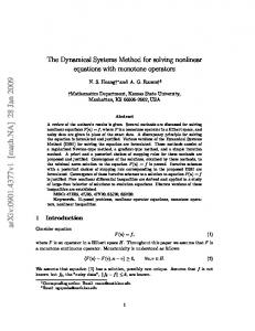
Traditional means of encoding trajectories is based on spline decomposition after averaging across training trajectories [7]– [10]. While this method is a useful tool for quick and efficient decomposition and generalization over a given set of trajectories, it is however heavily dependent on heuristics for segmenting and aligning the trajectories and gives a poor estimate of nonlinear trajectories. Some alternatives to spline-based techniques perform regression over a nonlinear estimate of the motion based on Gaussian kernels [2], [11], [12]. These methods provide powerful means for encoding arbitrary multi-dimensional nonlinear trajectories. However, similar to spline-encoding, these approaches depend on explicit time-indexing and virtually operate in an open-loop. Time dependency makes these techniques very sensitive to both temporal and spatial perturbations. To compensate for this deficiency4, one requires a heuristic to re-index the new trajectory in time, while simultaneously optimizing a measure of how good the new trajectory follows the desired one. Finding a good heuristic is highly taskdependent and a non trivial task, and becomes particularly non intuitive in high-dimensional state spaces. Reference [13] proposed an EM algorithm which uses an (extended) Kalman smoother to follow a desired trajectory from the demonstrations. They use dynamic programming to infer the desired target trajectory and a time-alignment of all demonstrations. Their algorithm also learns a local model of the robot’s dynamics along the desired trajectory. Although this algorithm is shown to be an efficient method for learning complex motions, it is time dependent and thus shares the disadvantages mentioned above. Dynamical systems (DS) have been advocated as a powerful alternative to modeling robot motions [5], [14]. Existing approaches to the statistical estimation of f in Eq. 2 use either Gaussian Process Regression (GPR) [15], Locally Weighted Projection Regression (LWPR) [16], or Gaussian Mixture Regression (GMR) [14] where the parameters of the Gaussian Mixture are optimized through Expectation Maximization (EM) [17]. GMR and GPR find a locally optimal model of fˆ by maximizing the likelihood that the complete model represents the data well, while LWPR minimizes the meansquare error between the estimates and the data (for detailed discussion on these methods see [18]). Because all of the aforementioned methods do not optimize under the constraint of making the system stable at the attractor, they are not guaranteed to result in a stable estimate of the motion. In practice, they fail to ensure global stability and they also rarely ensure local stability of fˆ (see Definition 1). Such estimates of the motion may hence converge to spurious attractors or miss the target (diverging/unstable behavior) even when estimating simple motions such as motions in the plane, see Fig. 3. This is due to the fact that there is yet no generic theoretical solution to ensuring stability of arbitrary nonlinear autonomous DS [19]. Fig. 3 illustrates an example of unstable estimation of a nonlinear DS using the above three methods for learning a two dimensional motion. Fig. 3(a)

3

ξ1

ξ1

Fig. 3. An example of two-dimensional dynamics learned from three demonstrations using five different methods: GMR, LWPR, GPR, BM, and SEDS (this work). For further information please refer to the text.

represents the stability analysis of the dynamics learned with GMR. Here in the narrow regions around demonstrations, the trajectories converge to a spurious attractor just next to the target. In other parts of the space, they either converge to other spurious attractors far from the target or completely diverge from it. Fig. 3(b) shows the obtained results from LWPR. All trajectories inside the black boundaries converge to a spurious attractor. Outside of these boundaries, the velocity is always zero (a region of spurious attractors) hence a motion stops once it crosses these boundaries or it does not move when it initializes there. Regarding Fig. 3(c), while for GPR trajectories converge to the target in a narrow area close to demonstrations, they are attracted to spurious attractors outside that region. In all these examples, regions of attractions are usually very close to demonstrations and thus should be carefully avoided. However, the critical concern is that there is not a generic theoretical solution to determine beforehand whether a trajectory will lead to a spurious attractor, to infinity, or to the desired attractor. Thus, it is necessary to conduct numerical stability analysis to locate the region of attraction of the desired target which may never exist, or be very narrow. The Dynamic Movement Primitives (DMP) [20] offers a method by which a non-linear DS can be estimated while ensuring global stability at an attractor point. Global stability is ensured through the use of linear DS that takes precedence over the non-linear modulation to ensure stability at the end

4

of the motion. The switch from non-linear to linear dynamics proceeds smoothly according to a phase variable that acts as an implicit clock. Such implicit time dependency requires a heuristics to reset the phase variable in the face of temporal perturbations. When learning from a single demonstration, DMP offers a robust and precise means of encoding a complex dynamics. Here, we take a different approach in which we aim at learning a generalized dynamics from multiple demonstrations. We also aim at ensuring time-independency, and hence robustness to temporal perturbations. Learning also proceeds from extracting correlation across several dimensions. While DMP learns a model for each dimension separately, we here model a single multi-dimensional model. The approach we propose is hence complementary to DMP. The choice between using DMP or SEDS to model a motion is application dependent. For example, when the motion is intrinsically timedependent and only a single demonstration is available, one may use DMP to model the motion. In contrast, when the motion is time-independent and when learning from multiple demonstrations, one may opt to use SEDS. For a more detailed discussion of these issues and for quantitative comparisons across time-dependent and time-independent encoding of motions using DS, the reader may refer to [5], [21]. In our prior work [14], we developed a hybrid controller composed of two DS working concurrently in end-effector and joint angle spaces, resulting in a controller that has no singularities. While this approach was able to adapt on-line to sudden displacements of the target or unexpected movement of the arm during the motion, the model remained time dependent because, similarly to DMP, it relied on a stable linear DS with a fixed internal clock. We then considered an alternative DS approach based on Hidden Markov Model (HMM) and GMR [22]. The method presented there is time-independent and thus robust to temporal perturbations. Asymptotic stability could however not be ensured. Sole a brief verification to avoid large instabilities was done by evaluating the eigenvalues of each linear DS and ensuring they all have negative real parts. As stated in [22] and as we will show in Section IV, asking that all eigenvalues be negative is not a sufficient condition to ensure stability of the complete system, see e.g. Fig. 5. In [21], [23] we proposed a heuristics to build iteratively a locally stable estimate of nonlinear DS. This heuristics requires one to increase the number of Gaussians and retrain the mixture using Expectation-Maximization iteratively until stability can be ensured. Stability was tested numerically. This approach suffered from the fact that it was not ensured to find a (even locally) stable estimate and that it did not give any explicit constraint on the form of the Gaussians to ensure stability. The model had a limited domain of applicability because of its local stability, and it was also computationally intensive, making it difficult to apply the method in highdimensions. In [18], we proposed an iterative method, called Binary Merging (BM), to construct a mixture of Gaussians so as to ensure local asymptotic stability at the target, hence the model can only applied in a region close to demonstrations (see Fig. 3(d)). Though this work provided sufficient conditions to

IEEE TRANSACTION ON ROBOTICS, VOL. ?, NO. ?, ? 2011

make DS locally stable, similarly to [23], it still relied on determining numerically the stability region and had a limited region of applicability. In this paper, we develop a formal analysis of stability and formulate explicit constraints on the parameters of the mixture to ensure global asymptotic stability of DS. This approach provides a sound ground for the estimation of nonlinear dynamical systems which is not heuristic driven and has thus the potential for much larger sets of applications, such as the estimation of second order dynamics and for control of multi-degrees of freedom robots as we demonstrate here. Fig. 3(e) represents results obtained in this paper. Being globally asymptotically stable, all trajectories converge to the target. This ensures that the task can be successfully accomplished starting from any point in the operational space without any need to re-index or re-scale. Note that the stability analysis we presented here was published in a preliminary form in [5]. The present paper extends largely this work by a) having a more depth discussion on stability, b) by proposing two objective functions to learn parameters of DS and comparing their pros and cons c) by having a more detailed comparison of the performance of the proposed method, BM, and three best regression methods for estimating motion dynamics, namely GMR, LWPR, and GPR, and d) by having more robot experiments. III. M ULTIVARIATE R EGRESSION We use a probabilistic framework and model fˆ via a finite mixture of Gaussian functions. Mixture modeling is a popular approach for density approximation [24], and it allows a user to define an appropriate model through a tradeoff between model complexity and variations of the available training data. Mixture modeling is a method, that builds a coarse representation of the data density through a fixed number (usually lower than 10) of mixture components. An optimal number of components can be found using various methods, such as the Bayesian Information Criterion (BIC) [25], the Akaike information criterion (AIC) [26], the deviance information criterion (DIC) [27], that penalize large increase in the number of parameters when it only offers a small gain in the likelihood of the model. While non parametric methods, such as Gaussian Process or variants on these, offer optimal regression [15], [28], they suffer from the curse of dimensionality. Indeed, computing the estimate regressor f grows linearly with the number of data points, making such an estimation inadequate for on-thefly recomputation of the trajectory in the face of perturbations. There exists various sparse techniques to reduce the sensitivity of these methods to the number of datapoints. However, these techniques either become parametric by predetermining the optimal number of datapoints [29], or they rely on a heuristic such as information gain for determining the optimal subset of datapoints [30]. These heuristics resemble that offered by the BIC, DIC or AIC criteria. Estimating f via a finite mixture of Gaussian functions, the unknown parameters of fˆ become the prior π k , the mean µk and the covariance matrices Σk of the k = 1..K Gaussian functions (i.e. θk = {π k , µk , Σk } and θ = {θ1 ..θK }). The

KHANSARI-ZADEH and BILLARD: LEARNING STABLE NON-LINEAR DYNAMICAL SYSTEMS WITH GAUSSIAN MIXTURE MODELS

µ =

!

&

k

Σ =

Σkξ Σkξξ ˙

Σkξξ˙ Σkξ˙

!

A3  + b3

(4)

n

,N Given a set of N demonstrations {ξ t,n , ξ˙t,n }Tt=0,n=1 , each t,n ˙t,n recorded point in the trajectories [ξ , ξ ] is associated with a probability density function P(ξ t,n , ξ˙t,n ):



1

_ = f^()

µkξ µkξ˙

k

h3 ()

h2 ()

h1 ()

hk ()

mean and the covariance matrix of a Gaussian k are defined by:

5

A1  + b1 1



3

2 A2  + b2

3 2



P3 _ = f^() = k=1 hk ()(Ak  + bk )



P(ξ t,n , ξ˙t,n ; θ) =

K X

k=1

P(k)P(ξ t,n , ξ˙t,n |k)

 ∀n ∈ 1..N (5) t ∈ 0..T n

where P(k) = π k is the prior and P(ξ t,n , ξ˙t,n |k) is the conditional probability density function given by: P(ξ t,n , ξ˙t,n |k) = N (ξ t,n , ξ˙t,n ; µk , Σk ) = t,n t,n k T k −1 t,n t,n k 1 √ 12d k e− 2 ([ξ ,ξ˙ ]−µ ) (Σ ) ([ξ ,ξ˙ ]−µ ) (2π)

(6)

|Σ |

˙ Taking the posterior mean estimate of P(ξ|ξ) yields (as described in [31]): ξ˙ =

K X

k=1

P(k)P(ξ|k) k −1 (µkξ˙ + Σkξξ (ξ − µkξ )) (7) PK ˙ (Σξ ) P(i)P(ξ|i) i=1

The notation of Eq. 7 can be simplified through a change of variable. Let us define:  k −1  Ak = Σkξξ  ˙ (Σξ )  bk = µkξ˙ − Ak µkξ   hk (ξ) = PKP(k)P(ξ|k) i=1

(8)

P(i)P(ξ|i)

Substituting Eq. 8 into Eq. 7 yields: ξ˙ = fˆ(ξ) =

K X

hk (ξ)(Ak ξ + bk )

(9)

k=1

First observe that fˆ is now expressed as a nonlinear sum of linear dynamical systems. Fig. 4 illustrates the parameters of Eq. 8 and their effects on Eq. 9 for a 1-D model constructed with 3 Gaussians. Here, each linear dynamics Ak ξ + bk corresponds to a line that passes through the centers µk with slope Ak . The nonlinear weighting terms hk (ξ) in Eq. 9, where 0 < hk (ξ) ≤ 1, give a measure of the relative influence of each Gaussian locally. Observe that due to the nonlinear weighting terms hk (ξ), the resulting function fˆ(ξ) is nonlinear and is flexible enough to model a wide variety of motions. If one estimates this mixture using classical methods such as EM, one cannot guarantee that the system will be asymptotically stable. The resulting nonlinear model fˆ(ξ) usually contains several spurious attractors or limit cycles even for a simple 2D model (see Fig. 3). Next we determine sufficient conditions on the learning parameters θ to ensure asymptotic stability of fˆ(ξ).

Fig. 4. Illustration of parameters defined in Eq. 8 and their effects on fˆ(ξ) for a 1-D model constructed with 3 Gaussians. Please refer to the text for further information.

IV. S TABILITY A NALYSIS Stability analysis of dynamical systems is a broad subject in the field of dynamics and control, which can generally be divided into linear and nonlinear systems. Stability of linear dynamics has been studied extensively [19], where a linear DS can be written as: ξ˙ = Aξ + b (10) Asymptotic stability of a linear DS defined by Eq. 10 can be ensured by solely requiring that the eigenvalues of the matrix A be negative. In contrast, stability analysis of nonlinear dynamical systems is still an open question and theoretical solutions exist only for particular cases. Beware that the intuition that the nonlinear function fˆ(ξ) should be stable if all eigenvalues of matrices Ak , k = 1..K, have strictly negative real parts is not true. Here is a simple example in 2D that illustrates why this is not the case and also why estimating stability of nonlinear DS even in 2D is non-trivial. Example: Consider the parameters of a model with two Gaussian functions to be: " #  3 0   Σ1ξ = Σ2ξ =   0 3   " # " # (11) −3 −30 −3 3 1 2  Σξξ , Σξξ  ˙ = ˙ =  3 −3 −30 −3     1 2 1 2 µξ = µξ = µξ˙ = µξ˙ = 0 Using Eq. 8 we have: " # " #   −1 1 A1 = −1 −10 , A2 = 1 −1 −10 −1   1 2 b =b =0

(12)

The eigenvalues of the two matrices A1 and A2 are complex with values −1 ± 3.16i. Hence, each matrix determines a stable system. However, the nonlinear combination of the two matrices as per Eq. 9 is stable only when ξ2 = ξ1 , and is unstable in Rd \ {(ξ2 , ξ1 )|ξ2 = ξ1 } (see Fig. 5). Next we determine sufficient conditions to ensure global asymptotic stability of a series of nonlinear dynamical systems given by Eq. 7.

6

IEEE TRANSACTION ON ROBOTICS, VOL. ?, NO. ?, ? 2011

ξ˙ = A1 ξ

ξ˙ = h1 (ξ)A1 ξ + h2 (ξ)A2 ξ

ξ˙ = A2 ξ

10

dV dV dξ V˙ (ξ) = = dt dξ dt
1 d = (ξ − ξ ∗ )T (ξ − ξ ∗ ) ξ˙ 2 dξ = (ξ − ξ ∗ )T ξ˙ = (ξ − ξ ∗ )T fˆ(ξ)

ξ2

5 0

−5 −10

−5

0

5

−5

ξ1

0

5

ξ1

−5

0

5

ξ1

Fig. 5. While each of the subsystem ξ˙ = A1 ξ (Left) and ξ˙ = A2 ξ (Center) is asymptotically stable at the origin, a nonlinear weighted sum of these systems ξ˙ = h1 (ξ)A1 ξ + h2 (ξ)A2 ξ may become unstable (Right). Here the system remains stable only for points on the line ξ2 = ξ1 (drawn in black).

 Theorem 1 Assume that the state trajectory evolves according to Eq. 9. Then the function described by Eq. 9 is globally asymptotically stable at the target ξ ∗ in Rd if:

= (ξ − ξ ∗ )T

= (ξ − ξ ∗ )T = (ξ − ξ ∗ )T =

K X

k=1

(

(a) bk = −Ak ξ ∗ (b) Ak + (Ak )T ≺ 0

∀k = 1..K

(13)

where (Ak )T is the transpose of Ak , and . ≺ 0 refers to the negative definiteness of a matrix5 .

0

∀ξ ∈ Rd

(16)

0 (b) V˙ (ξ) < 0   (c) V (ξ ∗ ) = 0

&

∀ξ ∈ Rd & ξ 6= ξ ∗ ∀ξ ∈ Rd & ξ = 6 ξ∗ ∗ V˙ (ξ ) = 0

(14) ˙ However, since Note that V˙ is a function of both ξ and ξ. ξ˙ can be directly expressed in terms of ξ using Eq. 9, one can finally infer that V˙ only depends on ξ. Consider a Lyapunov function V (ξ) of the form: V (ξ) =

1 (ξ − ξ ∗ )T (ξ − ξ ∗ ) 2

∀ξ ∈ Rd

(15)

Observe first that V (ξ) is a quadratic function and hence satisfies condition Eq. 14(a). Condition given by Eq. 14(b) follows from taking the first derivative of V (ξ) with respect to time, we have: 5 A d × d real symmetric matrix A is positive definite if ξ T Aξ > 0 for all non-zero vectors ξ ∈ Rd , where ξ T denotes the transpose of ξ. Conversely A is negative definite if ξ T Aξ < 0. For a non-symmetric matrix, A is positive ˜ = (A + AT )/2 is (negative) definite if and only if its symmetric part A positive (negative) definite.

V˙ (ξ ∗ ) =

K X

k=1

h (ξ)(ξ − ξ ) A (ξ − ξ ) k

∗ T

k

(17)

∗

=0

(18)

ξ=ξ ∗

Therefore, an arbitrary ODE function ξ˙ = fˆ(ξ) given by Eq. 9 is globally asymptotically stable if conditions of Eq. 13 are satisfied.  Conditions (a) and (b) in Eq. 13 are sufficient to ensure that an arbitrary nonlinear function given by Eq. 9 is globally asymptotically stable at the target ξ ∗ . Such a model is advantageous in that it ensures that starting from any point in the space, the trajectory (e.g. a robot arm’s end-effector) always converges to the target. V. L EARNING G LOBALLY A SYMPTOTICALLY S TABLE M ODELS Section IV provided us with sufficient conditions whereby the estimate fˆ(ξ) is globally asymptotically stable at the target. It remains now to determine a procedure for computing unknown parameters of Eq. 9, i.e. θ = {π 1 ..π K ; µ1 ..µK ; Σ1 ..ΣK } such that the resulting model is globally asymptotically stable. In this section we propose a learning algorithm, called Stable Estimator of Dynamical Systems (SEDS), that computes optimal values of θ by solving an optimization problem under the constraint of ensuring the model’s global asymptotic stability. We consider two different candidates for the optimization objective function: 1) log-likelihood, and 2) Mean Square Error (MSE).

KHANSARI-ZADEH and BILLARD: LEARNING STABLE NON-LINEAR DYNAMICAL SYSTEMS WITH GAUSSIAN MIXTURE MODELS

The results from both approaches will be evaluated and compared in Section VI-A. SEDS-Likelihood: using log-likelihood as a means to construct a model. n

N T 1 XX log P(ξ t,n , ξ˙t,n |θ) min J(θ) = − θ T n=1 t=0

(19)

subject to   (a) bk = −Ak ξ ∗    k k T   (b) A + (A ) ≺ 0 k (c) Σ ≻ 0    (d) 0 < π k ≤ 1    (e) PK π k = 1 k=1

∀k ∈ 1..K

(20)

SEDS-MSE: using Mean Square Error as a means to quantify the accuracy of estimations based on demonstrations6. n

N T 1 X X ˆ˙t,n ˙t,n 2 min J(θ) = kξ − ξ k θ 2T n=1 t=0

Algorithm 1 Procedure to determine an initial guess for the optimization parameters n ,N Input: {ξ t,n , ξ˙t,n }Tt=0,n=1 and K 1: Run EM over demonstrations to find an estimate of π k , µk , and Σk , k ∈ 1..K. 2: Define π ˜ k = π k and µ ˜kξ = µkξ 3: Transform covariance matrices such that they satisfy the optimization constraints given by Eq. 20(b) and (c):  ˜ k = I ◦ abs(Σk ) Σ  ξ ξ    ˜ k = −I ◦ abs(Σk ) Σ ˙ ˙ ξξ ξξ ∀k ∈ 1..K ˜ k = I ◦ abs(Σk )  Σ  ξ˙ ξ˙   Σ ˜ k = −I ◦ abs(Σk ) ξ ξ˙

PN where P(ξ t,n , ξ˙t,n |θ) is given by Eq. 5, and T = n=1 T n is the total number of training data points. The first two constraints in Eq. 20 are stability conditions from Section IV. The last three constraints are imposed by the nature of the Gaussian Mixture Model to ensure that Σk are positive definite matrices, priors π k are positive scalars smaller or equal than one, and sum of all priors is equal to one (because the probability value of Eq. 5 should not exceed 1).

(21)

subject to the same constrains as given by Eq. 20. In Eq. 21, ˆ ξ˙t,n = fˆ(ξ t,n ) are computed directly from Eq. 9. Both SEDS-Likelihood and SEDS-MSE can be formulated as a Non-linear Programming (NLP) problem [32], and can be solved using standard constrained optimization techniques. We use a Successive Quadratic Programming (SQP) approach relying on a quasi-Newton method7 to solve the constrained optimization problem [32]. SQP minimizes a quadratic approximation of the Lagrangian function over a linear approximation of the constraints8 . 6 In our previous work [5], we used a different MSE cost function, that balanced the effect of following the trajectory and the speed. See Appendix A for a comparison of results using both cost functions and further discussion. 7 Quasi-Newton methods differ from classical Newton methods in that they compute an estimate of the Hessian function H(ξ), and thus do not require a user to provide it explicitly. The estimate of the Hessian function progressively approaches to its real value as optimization proceeds. Among quasi-Newton methods, we use Broyden-Fletcher-Goldfard-Shanno (BFGS) [32]. 8 Given the derivative of the constraints and an estimate of the Hessian and the derivatives of the cost function with respect to the optimization parameters, the SQP method finds a proper descent direction (if it exists) that minimizes the cost function while not violating the constraints. To satisfy equality constraints, SQP finds a descent direction that minimizes the cost function by varying the parameters on the hyper-surface satisfying the equality constraints. For inequality constraints, SQP follows the gradient direction of the cost function whenever the inequality holds (inactive constraints). Only at the hyper-surface where the inequality constraint becomes active, SQP looks for a descent direction that minimizes the cost function by varying the parameters on the hyper-surface or towards the in-active constraint domain.

7

4:

ξ ξ˙

where ◦ and abs(.) corresponds to entrywise product and absolute value function, and I is a d × d identity matrix. Compute µ ˜kξ˙ by solving the optimization constraint given by Eq. 20(a): ˜ k˙ (Σ ˜ k )−1 (˜ µ ˜kξ˙ = Σ µkξ − ξ ∗ ) ξ ξξ

˜ 1 ..Σ ˜K} Output: θ 0 = {˜ π 1 ..˜ πK ; µ ˜ 1 ..˜ µK ; Σ Our implementation of SQP has several advantages over general purpose solvers. First, we have an analytic expression of the derivatives, improving significantly the performances. Second, our code is tailored to solve the specific problem at hand. For example, a reformulation guarantees that the optimization constraints (a), (c), (d), and (e) of Eq. 20 are satisfied. There is thus no longer the need to explicitly enforce them during the optimization. The analytical formulation of derivatives and the mathematical reformulation to satisfy the optimization constraints are explained in details in [33]. Note that a feasible solution to these NLP problems always exists. Algorithm 1 provides a simple and efficient way to compute a feasible initial guess for the optimization parameters. Starting from an initial value, the solver tries to optimize the value of θ such that the cost function J is minimized. However since the proposed NLP problem is non-convex, one cannot ensure to find the globally optimal solution. Solvers are usually very sensitive to initialization of the parameters and will often converge to some local minima of the objective function. Based on our experiments, running the optimization with the initial guess obtained from Algorithm 1 usually results in a good local minimum. In all experiments reported in Section VI, we ran the initialization three to four times, and use the result from the best run for the performance analysis. We use the Bayesian Information Criterion (BIC) to choose the optimal set K of Gaussians. BIC determines a tradeoff between optimizing the model’s likelihood and the number of parameters needed to encode the data: BIC = T J(θ) +

np log(T ) 2

(22)

where J(θ) is the normalized log-likelihood of the model computed using Eq. 19, and np is the total number of free

8

IEEE TRANSACTION ON ROBOTICS, VOL. ?, NO. ?, ? 2011

parameters. The SEDS-Likelihood approach requires the estimation of K(1+3d+2d2 ) parameters (the priors π k , mean µk and covariance Σk are of size 1, 2d and d(2d+1) respectively). However, the number of parameters can be reduced since the constraints given by Eq. 20(a) provide an explicit formulation to compute µkξ˙ from other parameters (i.e. µkξ , Σkξ , and Σkξξ ˙ ). Thus the total number of parameters to construct a GMM with K Gaussians is K(1 + 2d(d + 1)). As for SEDS-MSE, the number of parameters is even more reduced since when constructing fˆ, the term Σkξ˙ is not used and thus can be omitted during the optimization. Taking this into account, the total number of learning parameters for the SEDS-MSE reduces to K(1 + 23 d(d + 1)). For both approaches, learning grows linearly with the number of Gaussians and quadratically with the dimension. In comparison, the number of parameters in the proposed method is fewer than GMM and LWPR9 . The retrieval time of the proposed method is low and in the same order of GMR and LWPR. The source code of SEDS can be downloaded from http:// lasa.epfl.ch/ sourcecode/ VI. E XPERIMENTAL E VALUATIONS Performance of the proposed method is first evaluated against a library of 20 human handwriting motions. These were chosen as they provide realistic human motions while ensuring that imprecision in both recording and generating motion is minimal. Precisely, in Section VI-A we compare the performance of the SEDS method when using either the likelihood or MSE. In Section VI-B, we validate SEDS to estimate the dynamics of motion of two robot platforms (a) the seven degrees of freedom (DOF) right arm of the humanoid robot iCub, and (b) the six DOF industrial robot Katana-T arm. In Sections VI-C and VI-D, we show that the method can learn 2nd and higher order dynamics and that allows to embed different local dynamics in the same model. Finally, in Section VI-E, we compare our method against those of four alternative methods GMR, LWPR, GPR, and BM. A. SEDS training: Likelihood vs. MSE In Section V we proposed two objective functions: likelihood and MSE for training the SEDS model. We compare the results obtained with each method for modeling 20 handwriting motions. The demonstrations are collected from pen input using a Tablet-PC. Fig. 6 shows a qualitative comparison of the estimate of handwriting motions. All reproductions were generated in simulation to exclude the error due to the robot controller from the modeling error. The accuracy of the estimate is measured according to Eq. 23, with which the method accuracy in estimating the overall dynamics of the underlying model fˆ is quantified by measuring the discrepancy between the direction and magnitude of the estimated and observed velocity vectors for all training data points10 . 9 The number of learning parameter in GMR and LWPR is K(1+3d+2d2 ) and 72 K(d + d2 ) respectively. 10 Eq. 23 measures the error in our estimation of both the direction and magnitude of the motion. It is hence a better estimate of how well our model encapsulates the dynamics of the motion, in contrast to a MSE on the trajectory alone.

TABLE I P ERFORMANCE COMPARISON OF SEDS-L IKELIHOOD AND SEDS-MSE IN LEARNING 20 HUMAN HANDWRITING MOTIONS

Method

Average/Range of error e¯

Average/Range of No. of Parameters

Average Training Time (sec)

SEDS-MSE

0.25 / [0.18-0.43]

50 / [20 - 70]

27.4 / [3.1-87.7]

SEDSLikelihood

0.19 / [0.11-0.33]

65 / [26 - 91]

19.2 / [2.2-48.3]

e¯ =

1 T

PN

n=1

 t=0 r(1 −

PT n

(ξ˙t,n )T ξˆ˙t,n )2 ˆ ˙ kξ t,n kkξ˙t,n k+ǫ

+

˙t,n ˆ˙t,n )T (ξ˙t,n −ξˆ˙t,n ) q (ξ k−ξ˙ξt,n kk ξ˙t,n k+ǫ

 12

(23)

where r and q are positive scalars that weigh the relative influence of each factor11 , and ǫ is a very small positive scalar. The quantitative comparison between the two methods is represented in Table I. SEDS-Likelihood slightly outperforms SEDS-MSE in accuracy of the estimate, as seen in Fig. 6 and Table I. Optimization with MSE results in a higher value of the error. This could be due to the fact that Eq. 21 only considers the norm of ξ˙ during the optimization, while when computing e¯ the direction of ξ˙ is also taken into account (see Eq. 23). Though one could improve the performance of SEDS-MSE by considering the direction of ξ˙ in Eq. 21, this would make the optimization problem more difficult to solve by changing a convex objective function into a non-convex one. SEDS-MSE is advantageous over SEDS-Likelihood in that it requires fewer parameters (this number is reduced by a factor of 21 Kd(d + 1)). On the other hand, SEDS-MSE has a more complex cost function which requires computing GMR at each iteration over all training datapoints. As a result the use of MSE makes the algorithm computationally more expensive and it has a slightly longer training time (see Table I). Following the above observations that SEDS-Likelihood outperforms SEDS-MSE in terms of accuracy of the reconstruction and the training time, in the rest of the experiments we will use only SEDS-Likelihood to train the global model12 . B. Learning Point-to-Point Motions in the Operational Space We report on five robot experiments to teach the KatanaT and the iCub robot to perform nonlinear point-to-point motions. In all our experiments the origin of the reference coordinates system is attached to the target. The motion is hence controlled with respect to this frame of reference. Such representation makes the parameters of a DS invariant to changes in the target position. In the first experiment, we teach a six degrees of freedom (DOF) industrial Katana-T arm how to put small blocks into 11 Suitable values for r and q must be set to satisfy the user’s design criteria that may be task-dependent. In this paper we consider r = 0.6 and q = 0.4. 12 Note that in our experiments the difference between the two algorithms in terms of the number of parameters is small, and thus is not a decisive factor.

KHANSARI-ZADEH and BILLARD: LEARNING STABLE NON-LINEAR DYNAMICAL SYSTEMS WITH GAUSSIAN MIXTURE MODELS

Target

Demonstrations

Reproductions

9

Initial points

ξ2

ξ2

Results from SEDS−Likelihood

ξ1

ξ1

ξ1

ξ1

ξ1

ξ1

ξ1

ξ1

ξ1

ξ1

ξ1

ξ1

ξ1

ξ1

ξ2

ξ2

Results from SEDS−MSE

ξ1 Fig. 6.

ξ1

ξ1

ξ1

ξ1

ξ1

Performance comparison of SEDS-Likelihood and SEDS-MSE through a library of 20 human handwriting motions.

a container13 (see Fig. 7). We use the Cartesian coordinates system to represent the motions. In order to have humanlike motions, the learned model should be able to generate trajectories with both similar position and velocity profiles to the demonstrations. In this experiment, the task was shown to the robot six times, and was learned using K = 6 Gaussian functions. Fig. 7(a) illustrates the obtained results for generated trajectories starting from different points in the task space. The direction of motion is indicated by arrows. All reproduced trajectories are able to follow the same dynamics (i.e. having similar position and velocity profile) as the demonstrations. Immediate Adaptation: Fig. 7(b) shows the robustness of the model to the change in the environment. In this graph, the original trajectory is plotted in thin blue line. The thick black line represents the generated trajectory for the case where the target is displaced at t = 1.5 second. Having defined the motion as autonomous Dynamical Systems, the adaptation to the new target’s position can be done instantly. Increasing Accuracy of Generalization: While convergence to the target is always ensured from conditions given by Eq. 13, due to the lack of information for points far from demonstrations, the model may reproduce some trajectories that are not consistent with the usual way of doing the task. For example, consider Fig. 8-Top, i.e. when the robot starts the motion from the left-side of the target, it first turns around the container and then approaches the target from its rightside. This behavior may not be optimal as one expects the robot to follow the shortest path to the target and reach it 13 The robot is only taught how to move blocks. The problem of grasping the blocks is out of the scope of this paper. Throughout the experiments, we pose the blocks such that they can be easily grasped by the robot.

from the same side as the one it started from. However, such a result is inevitable since the information given by the teacher is incomplete, and thus the inference for points far from the demonstrations are not reliable. In order to improve the task execution, it is necessary to provide the robot with more demonstrations (information) over regions not covered before. By showing the robot more demonstrations and re-training the model with the new data, the robot is able to successfully accomplish the task (see Fig. 8-Bottom). The second and third experiments consisted of having Katana-T robot place a saucer at the center of the tray and putting a cup on the top of the saucer. Both tasks were shown 4 times and were learned using K = 4 Gaussians. The experiments and the generalization of the tasks starting from different points in the space are shown in Fig. 9 and 10. Fig. 11 shows the adaptation of both models in the face of perturbations. Note that in this experiment the cup task is executed after finishing the saucer task; however, for convenience we superimpose both tasks in the same graph. In both tasks the target (the saucer for the cup task and the tray for the saucer task) is displaced during the execution of the task at the time t = 2 seconds. In both experiments, the adaptation to the perturbation is handled successfully. The forth and fifth experiments consisted of having the seven DOF right arm of the humanoid robot iCub perform complex motions, containing several nonlinearities (i.e. successive curvatures) in both position and velocity profiles. Similar to above, we use the Cartesian coordinates system to represent these motions. The tasks are shown to the robot by teleoperating it using motion sensors (see Fig. 1). Fig. 12 illustrates the result for the first task where the iCub starts

10

IEEE TRANSACTION ON ROBOTICS, VOL. ?, NO. ?, ? 2011

Target

Demonstrations

Trajectory of Reproductions

Reproductions Target

Velocity Profile of Reproductions

Old Demonstrations

New Demonstrations

Reproductions

(a) Generalization based on the original model 100

100

ξ3 (mm)

100 50 0

ξ3 (mm)

ξ˙3 (mm/s)

150 50

0

0 −100

−50 50

−100 0 −100 −200 −300 −400

−50

0 −50

ξ2 (mm)

ξ1 (mm)

80 60 40 20

ξ˙1 (mm/s)

−200

20 0

300

−20

0

200

100

ξ˙2 (mm/s)

150 100 50

0

−100

ξ1 (mm)

−200

0 −50

−300

ξ2 (mm)

Projection of Trajectories on ξ1− ξ2 and ξ1− ξ3 planes (b) Generalization after retraining the model with the new data

150 100

ξ3 (mm)

0

50

100

0

ξ3 (mm)

ξ2 (mm)

50

−50

−50 −400

−300

−200

−100

−100 −400

0

−300

ξ1 (mm)

−200

−100

0 −100

0

ξ1 (mm)

−200 300

(a) The ability of the model to reproduce similar trajectories starting from different points in the space. Reproduction without perturbation

Reproduction under perturbation

Trajectory of Reproductions

Velocity Profile of Reproductions

100

150 100 0

50 −100

ξ1 (mm)

−200

0 −50

−300

ξ2 (mm)

Fig. 8. Improving the task execution by adding more data for regions far from the demonstrations.

60

50 Change in the target position at t=1.5

0 −50 −100 0

−100

−200

−300

0 −10

ξ2 (mm)

20 0 −20

80 60 40 20

ξ˙1 (mm/s)

Target

20 0 ˙ −20 ξ2 (mm/s)

−40

Demonstrations

0

150 100 50 0 400

200

ξ1 (mm)

0

0

Reproductions Velocity Profile of Reproductions

Trajectory of Reproductions

ξ3 (mm)

ξ1 (mm)

30 20 10

40

ξ˙3 (mm/s)

ξ˙3 (mm/s)

100

ξ3 (mm)

200

−600 −400 −200

ξ2 (mm)

100 0 −100 300 200

ξ˙2 (mm/s)

(a)

100 −200

0

−100

100

0

ξ˙1 (mm/s)

(b)

(c)

(b) The ability of the model to adapt its trajectory on-the-fly to a change in the target’s position Fig. 9. The Katana-T arm performing the experiment of putting a saucer on Fig. 7. The Katana-T arm performing the experiment of putting small blocks a tray. into a container. Please see the text for further information.

C. Learning 2nd Order Dynamics So far we have shown how DS can be used to model/learn a demonstrated motion when modeled as a first order time-

Target

Demonstrations

Trajectory of Reproductions

Reproductions

ξ˙3 (mm/s)

Velocity Profile of Reproductions

150

ξ3 (mm)

the motion in front of its face. Then it does a semi-spiral motion toward its right-side, and finally at the bottom of the spiral, it stretches forward its hand completely. In the second task, the iCub starts the motion close to its left fore-hand. Then it does a semi-circle motion upward and finally brings its arm completely down (see Fig. 13). The two experiments were learned using 5 and 4 Gaussian functions, respectively. In both experiments the robot is able to successfully follow the demonstrations and to generalize the motion for several trajectories with different starting points. Similarly to what was observed in the three experiments with the Katana-T robot, the models obtained for the iCub’s experiments are robust to perturbations.

100

50 0 −50

50 −400 −200

0 −300

−200

−100

ξ2 (mm) (a)

0

0

ξ1 (mm)

200 100

ξ˙2 (mm/s) (b)

0

150

100

50

0

ξ˙1 (mm/s) (c)

Fig. 10. The Katana-T arm performing the experiment of putting a cup on a saucer.

KHANSARI-ZADEH and BILLARD: LEARNING STABLE NON-LINEAR DYNAMICAL SYSTEMS WITH GAUSSIAN MIXTURE MODELS

(a) Trajectory of Reproductions

Target Saucer: Adapted Traj. Saucer: Original Traj. Cup: Adapted Traj. Cup: Original Traj.

ξ3 (mm)

150 100 50 0 500

Change in the target position at t=2

0

−600 −400 −200

ξ1 (mm)

0

−500

ξ2 (mm)

(b) Velocity Profile for the saucer task

(c) Velocity Profile for the cup task

ξ˙3 (mm/s)

ξ˙3 (mm/s)

50 50 0 −50 −100 300

200

100

0

ξ˙2 (mm/s)

−200

−100

0 −50

150 100

0

50

ξ˙2 (mm/s)

ξ˙1 (mm/s)

0 −50

0

50

100

150

ξ˙1 (mm/s)

Fig. 11. The ability of the model to on-the-fly adapt its trajectory to a change in the target’s position.

Target

Demonstrations

Reproductions

Trajectory of Reproductions

150

400

Initial points

Velocity Profile of Reproductions

100

ξ˙3 (mm/s)

ξ3 (mm)

200 0 −200 −400 300

50 0 −50 −100 −150

200

50

ξ˙1 (mm/s)

100

ξ1 (mm)

0

−100

400

200

0 −50

−200

0

100

ξ2 (mm)

−100

0

ξ˙2 (mm/s)

Fig. 12. The first experiment with the iCub. The robot does a semi-spiral motion toward its right-side, and at the bottom of the spiral it stretches forward its hand completely.

Target

Demonstrations

Reproductions

Trajectory of Reproductions

400

200 100

300

ξ˙3 (mm/s)

ξ3 (mm)

Initial points

Velocity Profile of Reproductions

200 100

0 −100 −200 200

−300 0 0

0 −100

−200

ξ2 (mm)

−100 −200

ξ1 (mm)

−400 200

0 100

0

ξ˙2 (mm/s)

−100

ξ˙1 (mm/s)

−200

Fig. 13. The second experiment with the iCub. The robot does a semi-circle motion upward and brings its arm completely down.

11

invariant ODE. Though this class of ODE functions are generic enough to represent a wide variety of robot motions, they fail to accurately define motions that rely on second order dynamics such as a self-intersecting trajectory or motions for which the starting and final points coincide with each other (e.g. a triangular motion). Critical to such kinds of motions is the ambiguity in the correct direction of velocity at the intersection point if the model’s variable ξ considered to be only the cartesian position (i.e. ξ = x ⇒ ξ˙ = x). ˙ This ambiguity usually results in skipping the loop part of the motion. However, in this example, this problem can be solved if one defines the motion in terms of position, velocity, and acceleration, i.e. a 2nd order dynamics: x¨ = g(x, x) ˙

(24)

where g is an arbitrary function. Observe that any second order dynamics in the form of Eq. 24 can be easily transformed into a first-order ODE through a change of variable, i.e.: ( x˙ = v ⇒ [x; ˙ v] ˙ = f (x, v) (25) v˙ = g(x, v) Having defined ξ = [x; v] and thus ξ˙ = [x; ˙ v], ˙ Eq. 25 reduces to ξ˙ = f (ξ), and therefore can be learned with the methods presented in this paper. We verify the performance of both methods in learning a 2nd order motion via a robot task. In this experiment, the iCub performs a loop motion with its right hand, where the motion lies in a vertical plane and thus contains a self intersection point (see Fig. 14). Here the task is shown to the robot 5 times. The motion is learned with seven Gaussian functions with SEDS-Likelihood. The results demonstrate the ability of SEDS to learn 2nd order dynamics. By extension, since any n-th order autonomous ODE can be transformed into a first-order autonomous ODE, the proposed methods can also be used to learn higher order dynamics; however, at the cost of increasing the dimensionality of the system. If the dimensionality of a n-th order DS is d, the dimensionality of the transformed dynamics into a first order DS is n × d. Hence, increasing the order of the DS is equivalent to increasing the dimension of the data. As the dimension increases, the number of optimization parameters also increases. If one optimizes the value of these parameters based on using a quasi-Newton method, the learning problem indeed becomes intractable as the number of dimensions increases. As an alternative solution, one can define the loop motion in terms of both the Cartesian position x and a phase variable. The phase dependent DS has lower dimension (i.e. dimensionality of d+1) compared to the second order DS, and is more tractable to learn. However, as it is already discussed in Section II, use of the phase variable makes the system timedependent. Depending on the application, one may prefer to choose the system of Eq. 25 and learn a more complex DS, or to use its phase variable form which is time-dependent, but easier to learn. D. Encoding Several Motions into one Single Model We have so far assumed that a single dynamical system drives a motion; however, sometimes it may be necessary

12

IEEE TRANSACTION ON ROBOTICS, VOL. ?, NO. ?, ? 2011

Trajectory of Reproductions

E. Comparison to Alternative Methods

ξ2 = x2 (mm)

250 200 Target Demonstrations Reproductions Initial points

150 100 50 0 0

50

100

150

200

250

300

350

ξ1 = x1 (mm) Velocity Profile of Reproductions

Acceleration Profile of Reproductions 20

ξ˙4 = x ¨2 (mm/s2 )

ξ4 = x˙ 2 (mm/s)

50

0

−50 −60

−40

−20

0

20

40

10 0 −10 −20 −30 −40

Fig. 14.

−60

−40

−20

0

20

ξ˙3 = x ¨1 (mm/s2 )

ξ3 = x˙ 1 (mm/s)

Learning a self intersecting motion with a 2nd order dynamics.

ξ2

Target Demonstrations Reproductions

ξ1 Fig. 15. Embedding different ways of performing a task in one single model. The robot follow an arc, a sine, or a straight line starting from different points in the workspace. All reproductions were generated in simulation.

The proposed method is also compared to three of the best performing regression methods to date (GPR, GMR with EM and LWPR14 ) and our previous work BM on the same library of handwriting motions represented in Section VI-A (see Table II) and the robot experiments described in Sections VI-B to VI-D (see Table III). All reproductions were generated in simulation to exclude the error due to the robot controller from the modeling error. Fig. 3 illustrate the difference between these five methods on the estimation of a 2D motion. To ensure fairer comparison across techniques, GMR was trained with the same number of Gaussians as that found with BIC on SEDS. As expected, GPR is the most accurate method. GPR performs a very precise non-parametric density estimation and is thus bound to give optimal results when using all of the training examples for inference (i.e. we did not use a sparse method). However, this comes at the cost of increasing the computation complexity and storing all demonstration datapoints (i.e. higher number of parameters). GMR outperforms LWPR, by being more accurate and requiring less parameters. Both BM and SEDS-Likelihood are comparatively as accurate as GMR and LWPR. To recall, neither GPR, GMR nor LWPR ensure stability of the system (neither local nor global stability), and BM only ensures local stability, see Section II and Fig. 3. SEDS outperforms BM in that it ensures global asymptotic stability and can better generalize the motion for trajectories far from the demonstrations. In most cases, BM is more accurate (although marginally so). BM offers more flexibility since it unfolds a motion into a set of discrete jointwise partitions and ensures that the motion is stable locally within each partition. SEDS is more constraining since it tries to fit a motion with a single globally stable dynamics. Finally, in contrast to BM, SEDS also enables to encode stable models of several motions into one single model (e.g. see Section VI-D). VII. D ISCUSSION

to execute a single task in different manners starting from different areas in the space, mainly to avoid joint limits, task constraints, etc. We have shown an example of such an application in an experiment with the Katana-T robot (see Fig. 8). Now we show a more complex example and use SEDS-Likelihood to integrate different motions into one single model (see Fig. 15). In this experiment, the task is learned using K = 7 Gaussian functions, and the 2D demonstrations are collected from pen input using a Tablet-PC. The model is learned using SEDS-Likelihood and it is provided with all demonstration data-points at the same time without specifying the dynamics they belong to. Looking at Fig. 15 we see that all the three dynamics are learned successfully with a single model and the robot is able to approach the target following an arc, a sine function, or a straight line path respectively starting from the left, right, or top-side of the task space. While reproductions follow locally the desired motion around each set of demonstrations, they smoothly switch from one motion to another in areas between demonstrations.

AND

F UTURE W ORK

In this paper we presented a method for learning arbitrary discrete motions by modeling them as nonlinear autonomous DS. We proposed a method called SEDS to learn the parameters of a GMM by solving an optimization problem under strict stability constraint. We proposed two objective functions SEDS-MSE and SEDS-Likelihood for this optimization problem. The models result from optimizing both objective functions benefit from the inherent characteristics of autonomous DS, i.e. online adaptation to both temporal and spatial perturbation. However, each objective function has its own advantages and disadvantages. Using log-likelihood is advantageous in that it is more accurate and smoother than MSE. Furthermore, the MSE cost function is slightly more time consuming since it requires computing GMR at each iteration for all training datapoints. However, the MSE objective function requires fewer parameters than the likelihood 14 The source code of all the three is downloaded from the website of their Authors.

KHANSARI-ZADEH and BILLARD: LEARNING STABLE NON-LINEAR DYNAMICAL SYSTEMS WITH GAUSSIAN MIXTURE MODELS

13

TABLE II P ERFORMANCE COMPARISON OF THE PROPOSED METHODS AGAINST ALTERNATIVE APPROACHES IN LEARNING 20 HUMAN HANDWRITING MOTIONS Method

Stability Ensured?

Average / Range of error e¯

SEDS-Likelihood

Yes / Global

BM

Yes / Local

GMR LWPR GPR

Average / Range of No. of Parameters

Average / Range of Training Time (sec)

Average Retrieval Time (sec)

0.19 / [0.11 - 0.33]

65 / [26 - 91]

19.23 / [2.22 - 48.26]

0.00068

0.18 / [0.11 - 0.50]

98 / [56 - 196]

20.4 / [3.56 - 55.16]

0.0019

No

0.13 / [0.08 - 0.28]

75 / [30 - 105]

0.211 / [0.038 - 0.536]

0.00068

No

0.17 / [0.07 - 0.35]

609 / [168 - 1239]

2.49 / [1.51 - 4.01]

0.00054

52.42 / [22.84 - 142.27]

0.07809

No

0.04 / [0.02 - 0.07]

2190 / [1806 -

3006]†

˙ Hence the total number of required parameters GPR’s learning parameter is of order of d(d + 1); however, it also requires keeping all training datapoints to estimate the output ξ. is d(d + 1) + 2n ∗ d, where n is the total number of datapoints. †

TABLE III P ERFORMANCE COMPARISON OF THE PROPOSED METHODS AGAINST ALTERNATIVE APPROACHES IN LEARNING ROBOT EXPERIMENTS PRESENTED IN S ECTIONS VI-B AND VI-C. T HE RESULT FOR SEDS IS OBTAINED USING LIKELIHOOD AS THE OBJECTIVE FUNCTION . Error e¯ Experiment

No. of Parameters

Training Time (sec)

SEDS

BM

GMR

LWPR

GPR

SEDS

BM

GMR

LWPR

GPR

SEDS

BM

GMR

LWPR

Katana-Block

1.6355

0.6465

1.4071

1.2619

0.2746

78

81

90

3780

7980

128.5

167.3

1.487

9.082

GPR 701

Katana-Saucer

0.2962

0.2285

0.1622

0.2595

0.0167

52

243

60

252

6930

217.1

294.9

0.398

4.017

543.6

Katana-Cup

0.4673

0.3758

0.5886

0.5136

0.1414

52

189

60

1008

7872

91.31

156.7

0.285

6.382

748.4

iCub-Task 1

1.0305

1.4197

1.2950

1.7219

0.0440

65

297

75

840

9642

161.5

317.6

0.833

8.034

834.5

iCub-Task 2

1.6921

1.1434

1.5255

1.8328

0.0487

52

297

60

336

8166

13.6

164.3

0.414

6.354

1786

iCub-2nd Order

0.2381

0.1025

0.0867

0.0625

0.0432

287

1144

315

5250

8020

50.77

191.7

1.986

7.342

436.2

Multi Model

0.26

—

0.1846

0.1626

0.0878

91

—

105

630

9006

58.59

—

2.61

10.82

2026.8

one which may make the algorithm faster in higher dimensions or when higher number of components is used. None of the two methods are globally optimal as they deal with a non-convex objective function. However, in practice, in the 20 handwriting examples and the six robot tasks, we reported here, we found that SEDS approximation was quite accurate. An assumption made throughout this paper is that represented motions can be modeled with a first order timeinvariant ODE. While the nonlinear function given by Eq. 9 is able to model a wide variety of motions, the method cannot be used for some special cases violating this assumption. Most of the time, this limitation can be tackled through a change of variable (as presented in our experiments, see Fig. 14). The stability conditions at the basis of SEDS are sufficient conditions to ensure global asymptotic stability of non-linear motions when modeled with a mixture of Gaussian functions. Although our experiments showed that a large library of robot motions can be modeled while satisfying these conditions, these global stability conditions might be too stringent to accurately model some complex motions. For these cases, the user could choose local approaches such as Binary Merging (BM) to accurately model desired motions. While in Section VI-C we showed how higher order dynamics can be used to model more complicated movements, determining the model order is definitely not a trivial task. It relies on having a good idea of what matters for the task at hand. For instance, higher order derivatives are useful to control for smoothness, jerkiness, energy consumption and hence may be used if the task requires optimizing for such criteria. Incremental learning is often crucial to allow the user to refine the model in an interactive manner. At this point in time,

the SEDS training algorithm does not allow for incremental retraining of the model. If one was to add new demonstrations after training the model, one would have to either retrain entirely the model based on the combined set of old and new demonstrations or build a new model from the new demonstrations and merge it with the previous model15 . For a fixed number of Gaussians, the former usually results in having a more accurate model, while the latter is faster to train (because it only uses the new set of demonstrations in the training). Ongoing work is directed at designing an on-line learning version of SEDS whereby the algorithm optimizes the parameters of the model incrementally as the robot explores the space of motion. This algorithm would also allow for the user to provide corrections and hence to refine the model locally, along the lines we followed in [34]. Furthermore, we are currently endowing the method with the on-the-fly ability to avoid possible obstacle(s) during the execution of a task. We will also focus on integrating physical constraints of the system (e.g. robot’s joints limit, the task’s constraint, etc.) into the model so as to solve for this during our global optimization. Finally, while we have shown that the system could embed more than one motion and, hence account for different ways to approach the same target depending on where the motion starts in the workspace, we have still yet to determine how many different dynamics can be embedded in the same system. 15 Two GMM with K 1 and K 2 number of Gaussian functions can be merged into a single model with K = K 1 + K 2 Gaussian functions by 1 concatenating their parameters, i.e.: θ = {θ 1 ..θ K ..θ K }, where θ k = k k k {π , µ , Σ }. The resulting model is no longer (locally) optimal; however, it could be an accurate estimation of both models, especially when there is no overlapping between the two models.

14

IEEE TRANSACTION ON ROBOTICS, VOL. ?, NO. ?, ? 2011

VIII. S UMMARY Dynamical systems offer a framework that allows for fast learning of robot motions from a small set of demonstrations. They are also advantageous in that they can be easily modulated to produce trajectories with similar dynamics in areas of the workspace not covered during training. However, their application to robot control has been given little attention so far, mainly because of the difficulty of ensuring stability. In this work, we presented an optimization approach for statistically encoding a dynamical motion as a first order autonomous nonlinear ODE with Gaussian Mixtures. We addressed the stability problem of autonomous nonlinear DS, and formulated sufficient conditions to ensure global asymptotic stability of such a system. Then, we proposed two optimization problems to construct a globally stable estimate of a motion from demonstrations. We compared performance of the proposed method with current widely used regression techniques via a library of 20 handwriting motions. Furthermore, we validated the methods in different point-to-point robot tasks performed with two different robots. In all experiments, the proposed method was able to successfully accomplish the experiments in terms of high accuracy during reproduction, ability to generalize motions to unseen contexts, and ability to adapt on-the-fly to spatial and temporal perturbations. ACKNOWLEDGMENT This work was supported by the European Commission through the EU Project AMARSI (FP7-ICT-248311). The authors kindly thank Jan Peters for his insightful comments during the development of this work, and Eric Sauser for preparing the experimental setup with the iCub robot. A PPENDIX A C OMPARISON

TO THE COST FUNCTION DESCRIBED IN

[5]

In our previous work [5], we had used a different MSE cost function from that proposed in this paper that balanced the error in both position and velocity:

+ ωξ˙ kξˆ˙n (t) − ξ˙t,n k2

Weights

ωξ = 1 ωξ˙ = 0

ωξ = 1 ωξ˙ = 1

ωξ = 0 ωξ˙ = 1

Motion 1

1.3531

0.4620

0.3135

Motion 2

1.4407

1.0853

1.3161

Motion 3

0.3739

0.3254

0.8839

Motion 4

1.6242

1.6047

2.2410

From normalizing the effect of each term   ωξ˙ = 0.076 0.5638 ω ˙ = 0.924  ξ  ωξ˙ = 0.293 0.8652 ω ˙ = 0.707  ξ  ωξ˙ = 0.101 0.3853 ω ˙ = 0.899  ξ  ωξ˙ = 0.129 1.4952 ωξ˙ = 0.871

example when learning the 20 human hand-writing motions described in Section VI-A using the cost function given in Eq. 26 has yielded an average error of 0.23 (against an error of 0.25 when using only speed in the cost function, see Table I). Another difficulty we avoid when considering solely one term in our cost function is that related to determining adequate values for the weighting terms (in [5] their value were preset to 1). To illustrate this issue, we ran the optimization on four different handwriting motions by varying the weighting terms given to the velocity and position respectively. We report on the accuracy as defined in Eq. 23 for each of these runs in Table IV. The weighting terms in the forth columns of Table IV are obtained by normalizing the effect of the position and velocity terms. One sees that the advantage of using either of the velocity or position term is not clear cut. For instance, when modeling motion 1, using only the velocity term provides the best result. For motions 2 and 4 the model obtained from the normalized weighting terms are more accurate, and the motion 3 is more accurate when the both weights are set equal. In general, it is difficult to say, a priori, which weights will result in a more accurate model. This effect is due to the fact that when the weights are changed, the shape of the cost function changes as well in a nonlinear manner. R EFERENCES

n

N T 1 XX min J(θ) = ωξ kξˆn (t) − ξ t,n k2 + θ N n=1 t=0

TABLE IV E VALUATION OF THE EFFECT OF WEIGHTING TERMS ON THE MSE COST FUNCTION PRESENTED IN [5]



(26)

ξˆ˙n (t) = fˆ(ξˆn (t)) are computed directly from Eq. 9. P ξˆn (t) = ti=0 ξˆ˙n (i)dt generate an estimate of the corresponding demonstrated trajectory ξ n by starting from the same initial points as that demonstrated, i.e. ξˆn (0) = ξ 0,n , ∀n ∈ 1..N . ωξ and ωξ˙ are positive scalars weighing the influence of the position and velocity terms in the cost function. In contrast to the cost function proposed in this paper that assumes independency across datapoints (see Eq. 21), the above cost function propagates the effect of the estimation error at each time step along each trajectory. Considering only the error in speed removes these effects (i.e. less complex optimization) while yielding nearly similar performance. For

[1] S. Schaal, “Is imitation learning the route to humanoid robots?” Trends in Cognitive Sciences, vol. 3, no. 6, pp. 233–242, 1999. [2] D. Kulic, W. Takano, and Y. Nakamura, “Incremental learning, clustering and hierarchy formation of whole body motion patterns using adaptive hidden markov chains,” The Int. Journal of Robotics Research, vol. 27(7), pp. 761–784, 2008. [3] A. Billard, S. Calinon, R. Dillmann, and S. Schaal, Handbook of Robotics. MIT Press, 2008, ch. Robot Programming by Demonstration. [4] K. Dautenhahn and C. L. Nehaniv, The agent-based perspective on imitation. Cambridge, MA, USA: MIT Press, 2002, pp. 1–40. [5] S.-M. Khansari-Zadeh and A. Billard, “Imitation learning of globally stable non-linear point-to-point robot motions using nonlinear programming,” in Proc. IEEE/RSJ Int. Conf. on Intelligent Robots and Systems (IROS), 2010, pp. 2676–2683. [6] E. D. Sontag, “Input to state stability: Basic concepts and results,” in Nonlinear and Optimal Control Theory. Springer Berlin / Heidelberg, 2008, ch. 3, pp. 163–220. [7] J.-H. Hwang, R. Arkin, and D.-S. Kwon, “Mobile robots at your fingertip: Bezier curve on-line trajectory generation for supervisory control,” in Proc. IEEE/RSJ IROS, vol. 2, 2003, pp. 1444–1449. [8] R. Andersson, “Aggressive trajectory generator for a robot ping-pong player,” IEEE Control Systems Magazine, vol. 9(2), pp. 15–21, 1989.

KHANSARI-ZADEH and BILLARD: LEARNING STABLE NON-LINEAR DYNAMICAL SYSTEMS WITH GAUSSIAN MIXTURE MODELS

[9] J. Aleotti and S. Caselli, “Robust trajectory learning and approximation for robot programming by demonstration,” Robotics and Autonomous Systems, vol. 54, pp. 409–413, 2006. [10] A. Ude, “Trajectory generation from noisy positions of object features for teaching robot paths,” Robotics and Autonomous Systems, vol. 11, no. 2, pp. 113–127, 1993. [11] M. Muehlig, M. Gienger, S. Hellbach, J. Steil, and C. Goerick, “Task level imitation learning using variance-based movement optimization,” in IEEE Intl Conf. on Robotics and Automation (ICRA), 2009, pp. 1177– 1184. [12] K. Yamane, J. J. Kuffner, and J. K. Hodgins, “Synthesizing animations of human manipulation tasks,” ACM Transactions on Graphics, vol. 23, no. 3, pp. 532–539, 2007. [13] A. Coates, P. Abbeel, and A. Y. Ng., “Learning for control from multiple demonstrations,” in Proc. 25th Intl. Conf. on Machine Learning (ICML), 2008, pp. 144–151. [14] M. Hersch, F. Guenter, S. Calinon, and A. Billard, “Dynamical system modulation for robot learning via kinesthetic demonstrations,” IEEE Trans. on Robotics, pp. 1463–1467, 2008. [15] C. Rasmussen and C. Williams, Gaussian processes for machine learning. Springer, 2006. [16] S. Schaal, C. Atkeson, and S. Vijayakumar, “Scalable Locally Weighted Statistical Techniques for real time robot learning, ” Applied Intelligence - Special issue on Scalable Robotic Applications of Neural Networks, vol. 17, no. 1, pp. 49–60, 2002. [17] A. Dempster and N. L. D. Rubin, “Maximum likelihood from incomplete data via the EM algorithm,” Journal of the Royal Statistical Society B, vol. 39, no. 1, pp. 1–38, 1977. [18] S.-M. Khansari-Zadeh and A. Billard, “BM: An iterative algorithm to learn stable non-linear dynamical systems with Gaussian Mixture Models,” in Proc. Int. Conf. on Robotics and Automation (ICRA), 2010, pp. 2381–2388. [19] J. Slotine and W. Li, Applied Nonlinear Control. Prentice-Hall, 1991. [20] P. Pastor, H. Hoffmann, T. Asfour, and S. Schaal, “Learning and generalization of motor skills by learning from demonstration,” in Proc. Int. Conf. on Robotics and Automation (ICRA), 2009, pp. 1293–1298. [21] E. Gribovskaya, S. M. Khansari-Zadeh, and A. Billard, “Learning nonlinear multivariate dynamics of motion in robotic manipulators,” Int. Journal of Robotics Research, pp. 1–37, 2010. [22] S. Calinon, F. D’halluin, E. Sauser, D. Caldwell, and A. Billard, “Learning and reproduction of gestures by imitation: An approach based on Hidden Markov Model and Gaussian Mixture Regression,” IEEE Robotics and Automation Magazine, vol. 17:2, pp. 44–54, 2010. [23] E. Gribovskaya and A. Billard, “Learning nonlinear multi-variate motion dynamics for real-time position and orientation control of robotic manipulators,” in Proc. 9th IEEE-RAS Int. Conf. on Humanoid Robots, 2009, pp. 472 – 477. [24] G. McLachlan and D. Peel, Finite Mixture Models. Wiley, 2000. [25] G. Schwarz, “Estimating the dimension of a model,” Annals of Statistics, vol. 6, pp. 461–464, 1978. [26] H. Akaike, “A new look at the statistical model identification,” IEEE Trans. on Automatic Control, vol. 19, pp. 716–723, 1974. [27] D. J. Spiegelhalter, N. G. Best, B. P. Carlin, and A. van der Linde, “Bayesian measures of model complexity and fit,” Journal of the Royal Statistical Society, Series B (Statistical Methodology), vol. 64, pp. 583– 639, 2002. [28] D. Nguyen-Tuong, M. Seeger, and J. Peters, “Local Gaussian Process Regression for real time online model learning and control,” in Advances in Neural Information Processing Systems 21, 2009, pp. 1193–1200. [29] E. Snelson and Z. Ghahramani, “Sparse Gaussian Processes using pseudo-inputs,” in Advances in Neural Information Processing Systems 18, 2006, pp. 1257–1264. [30] M. Seeger, C. K. I. Williams, and N. D. Lawrence, “Fast forward selection to speed up sparse Gaussian Process Regression,” in Proc. Ninth Int. Workshop on Artificial Intelligence and Statistics, 2003. [31] D. Cohn and Z. Ghahramani, “Active learning with statistical models,” Artificial Intelligence Research, vol. 4, pp. 129–145, 1996. [32] M. S. Bazaraa, H. Sherali, and C. Shetty, Nonlinear programming: Theory and Algorithms, 3rd Edition, Ed. John Wiley & Sons, 2006. [33] S.-M. Khansari-Zadeh and A. Billard, “The derivatives of the SEDS optimization cost function and constraints with respect to its optimization parameters,” Ecole Polytechnique Federale de Lausanne, Tech. Rep., 2010. [Online]. Available: http://lasa.epfl.ch/publications/publications.php [34] B. D. Argall, E. Sauser, and A. Billard, “Tactile guidance for policy refinement and reuse,” in Proc. 9th IEEE Int. Conf. on Development and Learning (ICDL), 2010, pp. 7–12.

15

S.M. Khansari-Zadeh is PhD student in Robotics at the school of Engineering at EPFL. He received his BSc (2005) in Aerospace Engineering and MSc (2008) in Flight Dynamics and Control from department of Aerospace Engineering at Sharif University of Technology. His research interests include modeling, control, and stability analysis of nonlinear dynamics and using imitation learning to infer control policies for robot control.

Aude Billard is Associate Professor and head of the Learning Algorithms and Systems Laboratory at the school of Engineering at EPFL. She received her BSc (1994) and MSc (1995) in Physics from EPFL and her PhD in Artificial Intelligence (1998) from the University of Edinburgh.