Learning stable, regularised latent models of neural population ...

Learning stable, regularised latent models of neural population dynamics Lars Buesing, Jakob H. Macke and Maneesh Sahani Gatsby Computational Neuroscience Unit University College London, UK 17 Queen Square, London, WC1N 3AR, UK {lars,jakob,maneesh}@gatsby.ucl.ac.uk Running title: Stable, regularised models of population dynamics Abstract Ongoing advances in experimental technique are making commonplace simultaneous recordings of the activity of tens to hundreds of cortical neurons at high temporal resolution. Latent population models, including Gaussian-process factor analysis and hidden linear dynamical system (LDS) models, have proven effective at capturing the statistical structure of such data sets. They can be estimated efficiently, yield useful visualisations of population activity, and are also integral building-blocks of decoding algorithms for brain-machine interfaces (BMI). One practical challenge, particularly to LDS models, is that when parameters are learned using realistic volumes of data the resulting models often fail to reflect the true temporal continuity of the dynamics, and indeed may describe a biologically-implausible unstable population dynamic; that is, it may predict neural activity that grows without bound. We propose a method for learning LDS models based on expectation maximisation that constrains parameters to yield stable systems and at the same time promotes capture of temporal structure by appropriate regularisation. We show that when only little training data is available our method yields LDS parameter estimates which provide a substantially better statistical description of the data than alternatives, whilst guaranteeing stable dynamics. We demonstrate our methods using both synthetic data and extracellular multi-electrode recordings from motor cortex.

1

Introduction

Modern multi-cell recording techniques (Kipke et al., 2008, Kerr and Denk, 2008) make it possible to monitor the spiking activity of tens to hundreds of individual neurons at the same time. Such data can provide much-needed insight into the dynamics of neural populations and the computations they perform, but only if the data are paired with statistical tools that can reliably identify the nature and course of those processes (Yu et al. 2006, Churchland et al. 2007; see Brown et al. 2004, Schneidman et al. 2006, Pillow et al. 2008 for other examples of statistical models of population activity). Concretely, such statistical models can be used to gain insights into neural population coding (Pillow et al., 2008), to relate neural population dynamics to observed behaviour (Afshar et al., 2011), and to provide important building blocks of cortical brain-machine interfaces (Wu et al., 2006, Santhanam et al., 2009, Wu et al., 2009). Latent factor models (sometimes called state-space models) (Durbin et al., 2001, Brown et al., 1998, Smith and Brown, 2003, Briggman et al., 2005, Yu et al., 2006, Wu et al., 2006, Paninski et al., 2010) provide a flexible way to model shared variance and thus common network activity in cortical recordings (Macke et al., 2011). In a latent factor model, the dependent structure in the observations—here, the firing rates of a population of neurons over time—arises through the dependence of those observations on a set of unobserved or latent state variables. As such, these 1

models may loosely be thought to describe sources of common input that couple the activity of different neurons (Kulkarni and Paninski, 2007). This stands in contrast to models in which one measurement is taken to depend directly on another, for example by assuming a direct connection between the observed neurons. As many multi-cell recording techniques (particularly extracellular electrode arrays) sample a local cortical population only very sparsely, such direct connections between measured neurons may be rare. Instead, the firing of the recorded sample of neurons is likely to be coordinated because those neurons participate in the same network—receiving input from, and driving, thousands of other cells which are themselves recurrently coupled. In this view, the evolution of the latent factors serves to track the way in which the activity of this network influences the recorded population. Indeed, the trajectory of low-dimensional state variables provides a compact visualisation of the population activity, facilitating single-trial analyses of neural population dynamics (Churchland et al., 2007, Yu et al., 2009). In a hidden linear dynamical system (LDS) model the latent factors form a temporal Markov chain of Gaussian random variables, the conditional mean of each linearly dependent on the value of the previous one, and the observations then depend on these latent state values in a similar linear-Gaussian manner (Kalman and Bucy, 1961, Ghahramani and Hinton, 1996, Durbin et al., 2001). One advantage to these choices is that the models can be fit efficiently to data using spectral subspace identification (SSID) techniques (Katayama, 2005) or by likelihood maximisation, often implemented by the Expectation Maximisation (EM) algorithm (Dempster et al., 1977, Digalakis et al., 1993, Ghahramani and Hinton, 1996). LDS models have been used extensively in numerous engineering and control-applications as well as in neuroscience (Cheng and Sabes, 2006, Macke et al., 2011). One challenge to fitting an LDS model (or, indeed, any other sort of statistical model) to neural population recordings is that neurophysiological data tend to be noisy and relatively few. This leads to a danger of “overfitting”: that is, the estimated parameters of a complex model might reflect the noise in the data used for estimation, rather than their true underlying structure. For example, a sufficiently high-order polynomial curve can exactly reproduce any measured inputoutput relationship, but if the measurements were noisy we would not expect each wiggle of the resulting curve to reflect genuine structure. The risk of overfitting might be lessened by restricting the complexity of the model being fit. A simple model, with few degrees of freedom, must direct those degrees of freedom to capture the most salient features of the data. A first-order polynomial would capture just the overall linear trend of the input-output function. The hope is that such significant features reflect genuine structure, rather than noise. Unfortunately, this strategy carries the converse risk that the model may be insufficiently powerful to describe the essential process that underlies the data. A straight line fit is of little value if the true function is a symmetric parabola or absolute-value curve. For an LDS model complexity could be controlled by the number of latent factors assumed, or, equivalently, by the dimensionality of the latent space. A low-dimensional model may overfit less, but may also fail to capture all the shared variance of the data. A higher-dimensional model is more flexible, but prone to overfitting. Overfitting in a dynamical model can also lead to estimates of the hidden dynamics which are unstable (Chui and Maciejowski, 1996): Models with unstable dynamics can predict unrealistically large measured values—here, firing rates—and have variances which grow progressively with time. This situation is especially problematic in the case of BMI (Simeral et al., 2011, Wolpaw and Wolpaw, 2012). Practically, a model can usually be fit to only a very small number of training trials, but must work well for a long period. Overfitting in general, and instability in particular, in the estimated dynamical model may impair the robustness of a BMI decoder. A less drastic approach to containing overfitting than restricting the dimensionality of the model is known as regularisation. This involves adding new terms to the cost function that must be optimised to fit the parameters. These terms bias the optimum towards particular values of the parameters, thus effectively shaping the model class. In our polynomial example, such terms might penalise large coefficients in high-order terms without enforcing a strictly lower-order form. If the cost function is the parameter log-likelihood, then these extra terms in the cost function may usu2

ally be interpreted as expressing a prior belief about the parameter values. The cost function then changes from the likelihood to the log-posterior distribution on the parameters, and the optimum reflects the “maximum-a-posteriori” parameter estimate. The most common form of regularisation simply penalises large values of the parameters: a process sometimes called “shrinkage” (although that term is also used more generally). In probabilistic terms, this corresponds to a prior belief that parameter values are relatively small, with a prior usually centred on zero values. When applied to the LDS model such simple zero-directed shrinkage may have unintended consequences. In particular, small entries in the matrix governing dynamics favour short correlation timescales in the latent space and hence also in the observation space. This might not be appropriate for the system one is trying to model. Also, regularisation by itself does not necessarily guarantee that the learnt dynamics will be stable (but see Van Gestel et al. 2001). The LDS model has a long history in time-series modelling, and several fitting procedures have been proposed to return stable parameter values. Lacy and Bernstein give two methods for ensuring that dynamical systems fitted with subspace identification methods (Katayama, 2005) are stable (Lacy and Bernstein, 2002, 2003). In their first method (Lacy and Bernstein, 2002), they constrain the largest singular value of the dynamics matrix to be less than one. While this is a sufficient condition for stability, it is not a necessary condition (see section 2.1) in the context of SSID. Therefore, this method constrains the solution space more strongly than necessary, and may rule out solutions that exhibit strong transients corresponding to non-normal dynamical matrices. While the same authors (Lacy and Bernstein, 2003) have also introduced a second method which overcomes this limitation to some extent, it has been shown to yield inferior results in practice (Siddiqi et al., 2007). Siddiqi and colleagues introduced a new constraint-generation algorithm for fitting stable dynamical systems with SSID methods and report that their algorithms outperform previous approaches. However, in their work they did not include a prior on the dynamics matrix and therefore obtain unregularised parameter estimates. Furthermore, SSID algorithms tend to be less statistically efficient than maximum likelihood methods. An alternative approach to containing overfitting in probabilistic models (which we do not pursue in this paper), is to extend the probabilistic view of regularisation to the fully Bayesian approach in which point-estimates of the parameters are replaced by consideration of the full posterior distribution. For many latent variable models, including the latent LDS model, the posterior cannot be found analytically but may be approximated by samples or by deterministic methods such as variational inference (Beal, 2003). In the fully Bayesian approach there is no fitting of the parameters as such (although sometimes hyper-parameters describing the prior are fit by hierarchical maximum likelihood), and thus no overfitting. All possible values of the parameters are considered in proportion to their posterior probabilities. However, existing Bayesian methods for the LDS model (Beal, 2003) do not guarantee stability, and it is not clear how they might be modified to do so. A state-space model that is closely related to the LDS model is Gaussian process factor analysis (GPFA) (Yu et al., 2009). This model can be understood as a generalisation both of factor analysis (FA) and of the latent LDS. All three types of models describe a joint Gaussian distribution on the observations by specifying a linear-Gaussian dependence on Gaussian-distributed latent variables. In FA these variables are independent over time. In an LDS, they form a first-order Markov chain. In GPFA they are described by a more general Gaussian process (GP) prior (Rasmussen, 2004). If the covariance function, which shapes the GP prior, is chosen to be stationary the resulting GPFA model is automatically stable. In the most common use of GPFA the different latent dimensions are taken to be independent of one another, and to each exhibit temporal covariance that decays according to a squared-exponential function. These choices are useful for visualisation, yielding smooth latent trajectories, and make the model less prone to overfitting due to the compactness of the resulting parameterisation. However, they do not provide an explicitly dynamical model. In particular, many interesting forms of dynamics cannot be described by a group of independentlyevolving variables. The linear-Gaussian Markov chain underlying the LDS model also describes a joint Gaussian distribution on the latent state, but its parameterisation is better able to describe the form of underlying dynamics.

3

Our objective in this paper is to show how the parameters of a stable LDS model can be robustly estimated by regularised maximum-likelihood methods. We introduce a regularisation term (or prior) on the dynamics matrix that discourages overfitting and which at the same time favours smooth dynamics with long time constants unlike conventional shrinkage-based regularisation. In addition, our approach ensures that the resulting dynamics are stable, thereby ruling out biologically-implausible high firing rates and variances without sacrificing the flexibility of the LDS to model complex dynamics. Using multi-electrode recordings from primate motor cortex, we show that our approach does indeed yield a better statistical model of neural data. This observation holds good both for test-data likelihood and for the cross-prediction measure of model performance introduced with GPFA (Yu et al., 2009), and persists over a range of different latent dimensionalities and training set sizes. Appropriate regularisation of this sort may help to overcome the difficulties posed by limited data to both scientific and prosthetic applications. This paper is organised as follows. We first review linear dynamical systems and discuss equivalent parameterisations and stability of the dynamics. We then explain how one can modify the EM algorithm to constrain parameter fits to yield stable system dynamics, and how we use a penalty term to bias the dynamics towards having long timescales. Subsequently, we apply our methods to surrogate data with known ground-truth, as well as to multi-electrode recordings from motor cortex of behaving monkeys.

2 2.1

Methods Linear dynamical systems

This section reviews some well-known properties of LDS models (for more extensive background see, e.g., Durbin et al. 2001, Katayama 2005) and defines the notation adopted in the paper. Let y(t) ∈ Rq be a q-dimensional column vector of observations made at time t, and let Y denote the q × T matrix assembled from the set of such vectors obtained at discrete times {1, . . . , T }: Y = [y(1), . . . , y(T )]. In the LDS model observations made at different times are not independent. The dependence is modelled by introducing a set of latent variables x(t) ∈ Rn , one at each observation time. These are usually of smaller dimension n < q, and may be assembled into the n × T matrix X = [x(1), . . . , x(T )]. The time series X is modelled as a first-order linear autoregressive process with Gaussian innovations, and the observations y(t) are taken to depend on a linear function of x(t) parameterised by the loading matrix C and mean value d: x(t + 1) y(t)

= =

Ax(t) + ǫ(t) Cx(t) + d + η(t).

(1)

The matrix A is called the dynamics matrix as it parameterises the deterministic part of the temporal evolution of X. The random variables ǫ(t), η(t) as well as the initial latent position x(1) are taken to be Gaussian distributed: ǫ(t) η(t)

∼ ∼

N (0, Q) N (0, R)

x(1)

∼

N (x0 , Q0 ).

The matrix R is constrained to be diagonal so that all statistical dependence within the model results only from the influence of the latent factors. We denote the LDS parameters by Θ = (A, Q, x0 , Q0 , C, R, d). As the dynamics are linear and ǫ(t), η(t) and x(1) are normally distributed, the variables X, Y are jointly normal, as are all conditional and marginal distributions. This makes inference in the LDS model tractable. The spectrum of the matrix A determines whether or not the corresponding dynamical system is stable. Systems with spectral radius ρ(A) < 1, i.e. those for which all eigenvalues ρi of A have an absolute value less than 1, are (Lyapunov) stable. Unstable systems have various properties which 4

might be undesirable, e.g. the expected a priori (i.e., before taking observations into account) latent covariance Qt = E[x(t)x(t)⊤ ] − E[x(t)]E[x(t)⊤ ] diverges as t → ∞, implying that samples from an unstable LDS will tend to grow exponentially in time. Furthermore, once conditioned on observations over a limited range of times, both the conditional mean and variance of predicted future values of both latents and observations will diverge. In contrast, it can be shown that for all stable systems there exists a stationary distribution limt→∞ p(xt ). This guarantees that observation predictions do not diverge for stable systems: The predicted mean and covariance approach finite values as time increases. For stable systems, one can define the time constants τi of the dynamics according to the equation τi := −1/ log(ρi ), and the time-lagged covariances of the latent state variables E[x(t)x(t+ s)⊤ ] − E[x(t)]E[x(t + s)⊤ ] decay in proportion to exp(−s/τi ) for s → ∞. For any LDS, the instantaneous covariance Qt changes according to the relation Qt+1 = AQt A⊤ + Q. Hence, the covariance matrix Q∞ of the stationary distribution limt→∞ p(xt ) solves the following discrete time Lyapunov equation: Q∞

=

AQ∞ A⊤ + Q.

(2)

The converse also holds: if for all positive definite matrices Q ≻ 0 equation (2) has a positive definite solution Q∞ ≻ 0 then A is stable. In many applications only stable systems are of interest. For neural population recordings, it is natural to assume that the underlying system is stable, as, for example, firing rates or other measurements are expected to always be confined to some physiological range, and do not diverge as a function of time. It is therefore natural to constrain the dynamics matrix to be stable during the estimation process for this application. The set of stable n × n matrices however is not convex, giving rise to difficulties in estimating stable matrices A (Siddiqi et al., 2007). A possible solution to this problem is to optimise over a smaller convex subset of the stable matrices. One such subset is the set of all matrices with singular values (SVs) less than 1 (Lacy and Bernstein, 2002) (a constraint which we will write as σ(A) < 1). This set is convex and all matrices in it are stable (one way to show this is to explicitly construct a positive definite solution to (2), see e.g. (Katayama, 2005)). The SV constraint however is more conservative than the eigenvalue one. This can be seen by the following example. Consider an upper triangular matrix with all elements equal to 0.9. This matrix obviously has eigenvalues of 0.9 but it has SVs > 1 (for all n > 1). This matrix is non-normal: Its dynamics are stable but they exhibit a transient expansion in some dimensions for appropriate initial conditions. Stationary LDSs are a subset of stable LDSs, where the distribution of the initial position x(1) equals the stationary distribution, i.e. x0 = 0 and Q0 = Q∞ = Qt for any time t.

2.2

Maximum likelihood estimation

The LDS parameters Θ = (A, Q, x0 , Q0 , C, R, d) can be estimated by spectral methods (Katayama, 2005) or by maximum likelihood (ML) techniques. The ML estimator Θ∗ML is one which maximises the likelihood, or equivalently the log-likelihood L(Θ; Y ), function derived from the data: Θ∗ML

=

argmaxΘ L(Θ; Y ) = argmaxΘ log p(Y |Θ).

The ML parameter estimate for most latent variable models cannot be found in closed form, and is commonly obtained by the iterative EM algorithm (Dempster et al., 1977, Ghahramani and Hinton, 1996). This often makes ML estimation substantially slower than spectral methods. However, ML estimates are statistically efficient, and thus make better use of the limited data available in the neural context. We will therefore focus on ML and related techniques. We denote the model whose parameters are estimated by likelihood-maximisation as the ML-LDS solution. ML estimation is consistent and asymptotically efficient. However, estimating the LDS parameters Θ from limited training data might lead to various problems. On the one hand, as the number of parameters grows quadratically with the number of latent dimensions n, modelling limited data with high latent dimensionalities may result in severe overfitting and unstable systems. 5

On the other hand, LDSs with few latent dimensions, which are less prone to overfitting, might not be expressive enough to model complex dynamics.

2.3

Enforcing stability

Real physical and biological processes cannot grow without bound, and so in many modelling applications it is reasonable to require stability in an estimated LDS model. Indeed, the distribution of the data may even be expected to be stationary on time scales that are relevant for the application. However, even in such cases, a simple ML parameter estimate from limited data may identify an unstable system. It is thus desirable to modify the simple ML procedure so as to constrain the resulting model to stability. Here we propose such a modification, based on a re-parameterisation of the LDS model. Assume an LDS with parameters Θ = (A, Q, x0 , Q0 , C, R, d) which is stable, i.e. ρ(A) < 1. We note first that for any LDS, the parameters may be transformed to effect an arbitrary, invertible, linear mapping of the latent space without changing the resulting distribution over observables. More ˜ = (T AT −1 , T QT ⊤ , T x0 , T Q0 T ⊤ , CT −1 , R, d) gives rise to explicitly, any LDS with parameters Θ ˜ for all invertible T ∈ Rn×n . the same distribution over observables as Θ, ie. p(Y |Θ) = p(Y |Θ), Let Q∞ be the stationary latent covariance of the system described by parameters Θ, and let it have the eigendecomposition Q∞ = U SU ⊤ where U is an orthogonal matrix and S is diagonal. Q∞ exists by our assumption of stability, and we assume here that it is positive definite and thus ˜ for which the S is invertible1 . By setting T := S −1/2 U ⊤ we obtain a new set of parameters Θ, ˜ stationary latent covariance Q∞ is the identity matrix I. This equivalence allows us to restrict consideration of stable LDS models to only those whose stationary latent covariance matrix is the identity without losing generality. For any such model, it follows by setting Q∞ = I in equation (2) that Q

=

I − AA⊤ .

(3)

Thus the family of stable LDS models can be parameterised by the smaller tuple of parameters (A, x0 , Q0 , C, R, d) provided that I − AA⊤ ≻ 0, with the corresponding conventional parameterisation given by Θ = (A, I − AA⊤ , x0 , Q0 , C, R, d). This smaller set of parameters may be estimated by maximising the likelihood function L((A, I − AA⊤ , x0 , Q0 , C, R, d); Y ) with respect to (A, x0 , Q0 , C, R, d). This maximisation can be achieved (in a local sense) by the EM algorithm. The E-step, which requires finding the posterior p(X|Y, Θ) proceeds just as for an unconstrained LDS with Q set to I − AA⊤ . Similarly, the optimisations of all parameters except for A in the M-step also remain unchanged. The optimisation for A, however, is no longer simply quadratic in A, as it is in the standard LDS M-step. Instead, it must be optimised numerically, by gradient ascent (see Appendix for details). We refer to the model with parameters found by maximisation of this reparameterised likelihood as a stable- or S-LDS. By definition, stability represents a constraint on the eigenvalues of A. However, once the system has been transformed to set Q∞ = I, the stability constraint translates to a constraint on the singular values si of A as: I − AA⊤ ≻ 0 ⇔ 0 ≤ si < 1 , ∀i = 1, . . . , n, that is, the matrix on the left hand side is positive definite whenever all singular values of A are smaller than one. It is worth noticing that this constraint need not be enforced explicitly in the optimisation of the M-step, as the cost function for A now contains terms of the form 1 − log |I − AA⊤ | 2

n

=

−

1X log(1 − s2i ). 2 i=1

1 It is sufficient to assume positive definite innovations covariance Q ≻ 0. Under this assumption Q ∞ is also positive definite.

6

These terms arise as I − AA⊤ is the covariance of the innovation noise. They effectively act as log-barrier functions (see Boyd and Vandenberghe 2004) restricting the optimisation to stay within the set with σ(A) < 1, and therefore ensure that the constraint I − AA⊤ ≻ 0 is always guaranteed to hold. At first glance, this equivalence between the singular-value constraint on A and stability of the LDS might seem to contradict the earlier discussion of SSID, where the requirement for unitbounded singular values was said to be overly constraining (Lacy and Bernstein, 2002). This apparent discrepancy emerges from the different approaches to parameter estimation taken in the two methods. SSID begins by finding the subspace spanned by the latent process, and implicitly identifies the loading matrix C by spectral methods. The dynamics matrix is then found in a second step, with C fixed at this value. With C fixed, constraining A to have unit-bounded singular values is indeed overly restrictive. By contrast, in each M-step of the EM algorithm, the matrices A and C (along with other parameters) are estimated together. Now, as the singular value constraint is enforced on A, the unconstrained C adjusts to fit any stable LDS without loss of generality. (See the Appendix for a more detailed discussion of this point.) Thus the singular value constraint is less restrictive in the context of ML estimation than it is for SSID.

2.4

Regularisation

One common way to address concerns about overfitting from limited data is to add regularisation terms to the objective function L(Θ; Y ), often equivalent to finding the maximum a posteriori (MAP) parameter values under a suitable choice of prior distribution on the parameters. Here, we consider forms of regularisation appropriate to stable LDS models. The M-step update to find a new dynamics matrix A for an unconstrained LDS resembles the solution to a linear regression problem. As such, it is tempting to adopt the standard approach of “ridge regression” (also referred to as “shrinkage” or “weight decay”) which penalises large entries in the matrix. Generalising slightly, we might introduce an Lp penalty term and minimise the function: X 1 |Aij |p . (4) Ec(p) (Θ) = −L(Θ; Y ) + λA p ij With the usual ridge choice of p = 2, this minimisation corresponds to finding the MAP estimate under an independent zero-mean Gaussian prior on each element of A. We call a model with stable parameterisation, and with parameters found using such regularisation a “conventionally regularised, stable LDS” (cRS-LDS). For an LDS model constrained to be stable by equation 3, shrinkage in the matrix A is effectively accompanied by inflation of the elements of Q. Even without this coupling, shrinkage in A leaves the innovations process to dominate the variance of the latent state and results in a latent dynamical process with short correlation times τi —a point that is illustrated in the experiments below. Such a tendency may be at odds with a prior belief that the latent dynamics underlying the measured data should evolve smoothly (Turner and Sahani, 2007). To incorporate the prior belief that the dynamics will be temporally smooth, we introduce a Gaussian prior on A: p(A)

=

n n Y Y

N (Aij | δij , λ−1 A ),

(5)

i=1 j=1

where Konecker’s delta δij denotes the elements of the identity matrix I. This prior is equivalent to an L2 penalty term on the elements of A − I. The prior discourages deviations of A from the identity matrix which describes constant dynamics. Thus we can interpret this prior as penalising deviations of the dynamics from constancy, rather than from independence. Furthermore, the coupling of equation 3 now results in a simultaneous penalty on the variance of the innovations 7

process. As the experiments below confirm, this prior favours longer time constants in the underlying dynamics. A system learned with this smoothness prior and stability constraints will be called a “regularised, stable LDS” (RS-LDS). We also explored the possible benefits of additionally regularising the loading matrix C by introducing a standard Gaussian prior: p(C)

=

q Y n Y

N (Cij | 0, λ−1 C ).

(6)

i=1 j=1

This prior biases all elements of C towards 0. To yield sensible results the scale of the latent process has to be fixed: Otherwise, in an unconstrained LDS, shrinkage in C could be compensated by equivalent inflation in A, Q, Q0 , x0 without affecting the implied distribution over the observations. This would render the regulariser effectively futile, as it would only bias the system to pick a particular one of several parameterisations of the same underlying system (and, in fact, could lead to numerical instabilities). In our framework, it is easy to set the scale of x(t) by the above choice of Q∞ = I (or equivalently Q = I − AA⊤ ) and by setting x0 = 0, Q0 = I, i.e. by constraining the system to be stationary. Thus, a further advantage of this particular stability constraint is that it sets the absolute scale of the latent process, and therefore makes it possible to define priors over the observation matrix C. We determine the regularisation parameter λA by cross-validation. In experiments where we also regularise C we avoid joint cross-validation of the two parameters λA , λC by setting q

λC

=

1X (var(Yi,: ))1/2 λA , q i=1

(7)

where var(Yi,: ) is the empirical variance of dimension i of the data. Hence, λC is set to λA scaled by the average standard deviation of the data. The relation (7) is motivated by the following heuristics. In each M-step, both A and C are found by solving regression problems. A maps a signal xt with (asymptotically) unit variance onto a signal xt+1 which also has (asymptotically) unit variance. By contrast, C maps a unit variance signal onto Y whose components have the variances var(Yi,: ). Thus, the expected scale of the weights in C should be on the order of var(Yi,: )1/2 times the expected scale of A. This is the relative scale set by equation (7). Furthermore, this choice of regulariser also ensures that the impact of regularisation is independent of the absolute scale of measurement of Y —a rescaling of all elements of Y would lead to a rescaling of λC and thus the relative contribution of the likelihood and the prior would remain unchanged. In summary, we estimate the parameters of a stationary LDS with parameters Θ = (A, Q, x0 , Q0 , C, R, d) under the constraint Q = I − AA⊤ ≻ 0 using a constrained EM algorithm. For the parameters R and d (whose number does not scale with the latent dimensionality n) we use maximum likelihood estimates, while we use MAP estimates for the dynamics matrix A and we have investigated both ML and MAP estimates of C. The systems are abbreviated as RS-LDS and cRS-LDS depending on the prior over A. Unless stated otherwise, all experiments were carried out with L2 -regularisation.

3 3.1

Results Experiments with artificial data

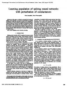
We sought first to contrast the results of learning within the stability-constrained parameterisation (S-LDS) to those of na¨ıve ML estimation. We sampled a time series of 100 time steps from a stable, stationary LDS model with n = 5 latent dimensions and q = 10 observed dimensions (for details see sections 5). The dynamics matrix A0 of the ground truth LDS had a spectral radius ρ(A0 ) = 0.95. Figure 1A shows 3 out of the 10 dimensions of the training data.

8

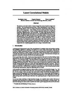
Using these samples as data, we estimated LDS parameters both by standard ML and ML with stability constraints as proposed in section 2.3. As mentioned above, unconstrained ML estimation of LDS parameters from small data sets may sometimes lead to unstable settings of the parameters. This is observed here. ML learning on the sampled training data yielded parameters ΘML that included an unstable dynamics matrix AML with ρ(AML ) = 1.007. We also trained an unregularised but stable LDS as described in section 2.3 on the same data and denote the resulting parameters as ΘS . The matrix AS was stable with ρ(AS ) = 0.998. Figure 1B, C shows example trajectories generated in the observation space by sampling from an LDS model with parameters ΘML (panel B) and ΘS (panel C). Although the spectral radius of AML seems only slightly greater than 1, samples from the corresponding LDS model grow substantially within only 200 time steps, illustrating the exponential growth in variance. By contrast, samples from the LDS model with ΘS stay close to the origin, showing that the corresponding stationary marginal distribution has finite mean and covariance. Indeed, the sample trajectory exhibits roughly the same variance as the training data; this is due to the fact that ΘS was learned under stability and stationarity constraints. A second numerical experiment on synthetic data explored the effects of adding a regularisation term (or, equivalently, a prior over the dynamics matrix) to the likelihood objective function. We repeatedly generated both a training data set and a separate test data set by sampling from a stationary LDS model with n = 5, q = 10 (see section 5 for details). The dynamics matrix of the generative model was chosen such that its spectrum had absolute values close to one and small imaginary parts (Figure 2A green crosses). For each run, we estimated LDS parameters from the training data both using standard ML estimation (ML-LDS), using our regularised, stable algorithm (RS-LDS) as well as using the conventionally regularised estimation (cRS-LDS). Insight into the behaviour of the different parameter estimates can be gained by studying the spectra of the resulting dynamics matrices, shown in Figure 2A (pooled over 40 runs). For little training data (2 trials, upper row), the eigenvalues in the ML-LDS spectrum (left column, blue circles) are often substantially smaller than the generative values (green crosses). They also show considerable scatter, sometimes approaching or crossing the unit circle, thus leading to instability as in Fig. 1. The introduction of a prior penalising deviations from the identity matrix drives the eigenvalues of the matrix found by RS-LDS (with a fixed regularisation parameter λA = 103 ) towards unity on the real line, whilst the stability constraint ensures that they all remain within the unit circle. The effects of these manipulations can be seen in the resulting spectra (Figure 2B, middle column, red circles). This results in estimates of eigenvalues that lie closer to 1 than ML estimates, with less downward bias and less scatter. However, a slight undershoot in the estimates of the larger imaginary parts is also evident. By contrast, the prior of cRS-LDS (right column, regularisation parameter λA = 103 ) drives the eigenvalues towards 0 (black circles). Thus the form of the prior is crucial. When the data are generated by a model with smooth dynamics, a prior favouring shorter timescales is unhelpful. With more training data (10 trials, lower row) all algorithms identify matrices with more accurate eigenvalue spectra, although the mismatched prior of cRS-LDS leads to slower convergence. This pattern of results in the eigenvalue spectrum is also reflected in the fit of the corresponding models to test data. Figure 2B shows the log-ratio between the likelihoods evaluated on the test data of the parameters estimated by the different algorithms and the true generative parameters as a function of the size of the training data set. Log-likelihood ratios that approach 0 reveal estimated parameters that provide as good a model of the test data as do the generative parameter values: that is, these parameters define a model that generalises well to new data. Smaller log-likelihood ratios suggest that the parameters have overfit the training data, capturing idiosyncratic features of those data and thus providing a poorer model of new data that do not share those features. We found that with increasing training data the likelihoods of models fit by both ML-LDS and RS-LDS converged to the likelihood of the generative parameters (bringing the log-ratios to 0). This convergence is theoretically expected and reflects both the consistency of ML estimates and the fact that MAP estimates under a fixed prior approach ML values as the number of available training data increase. Furthermore these results verify the robustness of the gradient9

based EM algorithm employed for RS-LDS estimation. For small training sets, the regularised RS-LDS approach yielded better models on test data than did the unregularised ML-LDS. This benefit shows the advantage of choosing an identity-centred prior when the true parameter values correspond to a smoothly evolving LDS model. This gain in generalisation, due to the reasonable accordance of the generative parameters with the RS-LDS prior, is also reflected in the tighter match of the ground truth eigenvalues and those identified by RS-LDS as shown in Figure 2A. Of course, this advantage of the RS-LDS prior depends crucially on the nature of the true generative process. For data sets which do not show high levels of temporal continuity, for which there is a mismatch between the RS-LDS prior and the data, no benefit is to be expected from RS-LDS estimates and other priors (e.g. those of cRS-LDS) might be more useful.

3.2

Application to multi-electrode recordings

The numerical experiments on artificial data have shown that the RS-LDS estimation approach yields stable and smooth dynamical system parameters, which generalise more accurately than do either na¨ıve ML or ML with conventional, shrinkage-based regularisation. Does RS-LDS estimation also lead to better models of real data? We fit LDS parameters to data collected during the execution of delayed reaches, using extracellular electrode arrays implanted in primate motor and premotor cortices. These data were collected by Churchland et al. (2006), who generously made them available for this study. The data used here included 105 units recorded for 56 trials, each 2.02 s long. Data acquisition and pre-processing are outlined briefly in the Appendix. We assessed how well models with the different parameters captured the statistical structure of the recorded neural population activity. To do so, we used two different cross-validated measures: the likelihood, expressed as the logarithm of its ratio with respect to that of a baseline model, and a firing-rate cross-prediction performance measure introduced by Yu et al. (2009) (details in the Appendix). The latter measure quantifies the ability of a model to predict the activity of one held-out unit given the activity of all the other units. As we are interested primarily in the generalisation performance of the models, performance was always measured on test data—i.e., data which had not been used to estimate the parameters. Figure 3 shows both performance measures for a variety of parameter estimation methods and models, as a function of the latent dimensionality n, using a small data set of 10 trials. We found that when models had more than 5 latent dimensions the RS-LDS parameters outperformed the ML ones by a significant margin in terms of both test likelihood and cross-prediction performance. Furthermore, these higher-dimensional models also outperformed the more restrictive lower-dimensional ones, so the benefits obtained by RS-LDS estimation in this regime contribute crucially to building more accurate models of the shared variance in the neural data. Interestingly, the precise value of the regularisation parameter λA had little effect on RSLDS performance. Figure 3 shows performance both with a fixed value of λA = 103 , as well as that obtained when the regularisation parameter was determined by cross-validation separately for each latent dimensionality, n. The two are barely different. We found this robustness to be generally true for the data studied here. The value λA = 103 was effective across different latent dimensionalities and cross-validation splits. We also investigated the performance of a stable LDS model with parameters estimated under regularisation of both A and C. The results show only a modest increase in performance when C was also regularised. This indicates that for the data at hand it is more important to regularise the dynamics matrix A, than to regularise the elements of C. In general, the number of degrees of freedom in A grows quadratically with n, whilst the number of elements of C only grows linearly with n. Hence, one would expect regularisation of A to be more important for larger latent dimensionalities. We also established that jointly cross-validating λA and λC does not increase performance noticeably in comparison to using the fixed relation given by eq. (7) (data not shown). The results also show that conventional shrinkage-based regularisation of the dynamics matrix (cRS-LDS) yields similar (or perhaps slightly inferior) results to unregularised ML on the real

10

neural data. This similarity is unsurprising, as cross-validation favours very small regularisation strengths λA for the shrinkage prior, making the regularised cost function essentially equivalent to the likelihood. (The residual and inconsistent small differences in test likelihood seem to result from an interaction between the stability-constraining reparameterisation of cRS-LDS and the parameter settings chosen to initialise EM.) The fact that the shrinkage prior confers no gain in quality of fit suggests that it is a poor match to the neural data, and that these data are better modelled by parameters that capture smoothness. This hypothesis is supported by inspection of the spectra of the estimated dynamics matrices (Figure 4A, showing eigenvalues of A for n = 15 pooled over four cross-validation folds for ML-LDS and RS-LDS with λA = 103 ). RSLDS, which offers the better statistical description of the data as assessed by test likelihood and cross-prediction performance has eigenvalues with absolute values close to 1 and small imaginary parts describing smooth temporal dynamics. By contrast, a considerable fraction of eigenvalues for the ML-estimated dynamics matrix have absolute values close to zero or have relatively large imaginary parts yielding temporally uncorrelated dynamics or fast oscillations respectively. These features appear not to improve the generalisation of the model. This relative lack of smoothness in the ML-LDS models is also visible in the trajectories of Figure 4B. Shown are three latent dimensions of the smoothed latent trajectories E[x(t)|Y, Θ] which are most likely for one 2.02 s trial of test data (the model was fit with n = 15 latent dimensions, with the top three orthonormalised projections shown, see Appendix). Trajectories such as these are often used for visualisation and are helpful for analyzing single trial effects (see Yu et al. 2009) in neural population recordings. The smoother trajectories of RS-LDS are also more accurate. They are derived from models with higher likelihood on the data, and make more accurate firing rate cross-predictions than trajectories derived from alternative models Figure 3. Furthermore, smoother trajectories may be preferable for visualisation as they allow the observer to focus on the structure exhibited by the data on behavioral time scales, without being distracted by rapid, possibly noisy, fluctuations. Regularisation is most effective when parameters must be estimated from relatively little training data. As more data become available, the ML parameter estimates overfit less severely, and— asymptotically—become statistically efficient. This phenomenon was visible in Figure 2A for an artificial data set. In order to determine the range of training set sizes where regularisation is beneficial we studied the performance of the different fitting approaches as a function of the training data size. The results are shown in Figure 5. RS-LDS with n = 20 and a fixed regularisation parameter λA = 103 outperformed ML-LDS with n = 10, 15, 20 for training sets consisting of 5 up to 30 trials; the complete dataset had 56 trials. In addition to L2 -regularisation we investigated the use of L1 -regularisation of A as well as of both A and C (and all combinations of L1 and L2 ). L1 -regularisation, related to LASSO regression, often leads to estimated parameters which are sparse in the sense that many estimated matrix elements are exactly 0 (or 1, for the diagonal elements of the identity-regularised A matrix). We found that L2 -regularisation performed better than L1 -regularisation on the data considered here, for all latent dimensionalities and training set sizes—although not by a large margin. Thus, there was little evidence that sparsity was a helpful prior in LDS models of neural data. In another experiment we added the constraint that the matrix A be diagonal to both ML and RS-LDS estimates. The resulting parameters performed more poorly than the ML parameters with optimal latent dimensionality, and worse than RS-LDS for all dimensionalities. These results held for all the training set sizes we investigated. This indicates that although the RS-LDS gains performance by penalising large off-diagonal elements of A, some non-zero values off the diagonal are essential to describe the structure of the latent dynamics underlying neural populations. Figure 3B also shows the cross-prediction performance of GPFA and of LDS models with parameters learned by the stable subspace identification (SSID) algorithm introduced by Siddiqi et al. (2007). For the latter we report for each dimensionality the performance obtained by choosing the optimal size of the Hankel matrix. Both methods perform substantially worse than RS-LDS for all dimensionalities. It needs to be emphasised, however, that the trial structure of the multi-electrode recordings analysed here is unsuitable for SSID algorithms, which assume a single 11

continuous time series instead of multiple trials. Furthermore, iterative, EM-based algorithms are much slower than SSID algorithms. We did not include either GPFA or SSID in Figure 3A as their likelihoods were substantially lower than those of the ML parameters for all model dimensionalities.

4

Discussion

In this study we have proposed two enhancements to parameter estimation in the standard LDS model, and tested the value of both in building models of neural population data. These enhancements reparameterise the innovations term of the LDS model so as to constrain it to remain stable, and provide a natural regularisation scheme that promotes smoothness within the latent dynamics. Both enhancements improved the quality of fit on the motor cortical data we studied—judged both by test-data likelihood and by leave-one-neuron-out cross-prediction—over na¨ıve ML estimation, conventional shrinkage-based regularisation, as well as stable SSID-based methods (Siddiqi et al., 2007). The gain in performance extended across models of various latent dimensionalities and was robust to the exact choice of the regularisation parameter. As might be expected, the benefit of regularisation was largest when the least data were used to estimate parameter values. However, the gains extended, albeit weakly, to larger data sets as well, and at no point did the RS-LDS approach perform more poorly than any of the alternatives we evaluated. Latent factor models of neural population firing seek to capture the shared population-level activity in a low-dimensional set of latent variables. To the extent that the concerted action of the population has the greatest impact on downstream processing, we might expect these latent variables to reflect the essence of the computational action of the population. The relative advantage in goodness-of-fit seen with smoothness-based regularisation over both conventional shrinkage and na¨ıve ML suggests that this shared element of motor cortical population activity does indeed evolve smoothly during the preparation and execution of instructed reaching movements. The most successful RS-LDS-estimated models exhibited long time scales stretching from several hundred milliseconds up to seconds, with relatively little shared variance at shorter timescales. Findings such as these hint at an underlying robust organisation of computation within neural populations, where short-time local fluctuations in firing are smoothed away across the population, leading to a more robust computational strategy. Appropriate regularisation schemes may also prove helpful for offline or online decoding of arm or hand trajectories from motor cortex recordings. State-of-the-art decoding performance is often achieved by decoders that are trained for specific experimental conditions (Gilja et al., 2011) and which often have to be re-trained for every session due to non-stationarity of the data on long time scales on the order of hours or days (Gilja et al., 2011). This limits the amount of available training data and renders appropriate regularisation worthwhile. However, it remains to be seen if the methods described here will benefit decoding performance in practical a BMI setting. A linear autoregressive process with Gaussian noise, such as the process governing the latent variable of an LDS model, is a special case of a Gaussian process (GP). Thus, the LDS latent model is related to Gaussian process factor analysis (GPFA), which is a state space model with an independent general GP prior on each latent variable trajectory (Yu et al., 2009). GPFA requires the specification of a covariance function that parameterises the evolution of the latent variables. This function is most often taken to be squared-exponential, a choice which yields particularly smooth latent variable trajectories. The alternative choice of a stationary absolute-exponential function (also known as the Ornstein-Uhlenbeck or OU covariance function) would yield a GP prior that corresponded precisely to a restricted stationary LDS in which both the dynamics matrix A and the innovations covariance Q were diagonal. This restriction reflects the assumption of GPFA that the different latent dimensions evolve independently under the prior. Thus, the stable LDS model can be seen as both a restriction and a generalisation of GPFA, which constrains the latent dynamics to be stable and Markovian (as with the OU covariance function) but allows for coupling between the latent dimensions via off-diagonal elements of the dy-

12

namics matrix. We showed that this parameterisation when combined with a suitable regulariser, yielded better performance than both GPFA with squared-exponential covariance functions, and an LDS model with diagonal dynamics matrix (equivalent to GPFA with an OU covariance function). At the same time, the latent trajectories obtained are smooth, by contrast to those found using ML estimation in an LDS. Thus, the current model arguably combines the advantages of squared-exponential GPFA (namely, stable and smooth dynamics) with those of linear dynamical systems (namely, a richer set of dynamics, as well as training time which is linear in the length of the trials). To our knowledge, the stability-constraining reparameterisation developed here has not been discussed previously in the context of ML-estimation of multi-dimensional LDS models. However, a similar parameterisation of a univariate LDS has been previously been exploited to build a probabilistic formulation of Slow Features Analysis (Turner and Sahani, 2007). The algorithm for learning stable, regularised LDSs proposed here also has some shortcomings. Although the performance turned out not to be very sensitive to fining tuning of the regularisation parameter, its order of magnitude still needs to be set, for example by cross-validation. In principle, one might seek to build a hierarchical model in which the distribution on the parameters could itself be learnt from data. This Bayesian approach was taken for the general LDS model by Beal (2003). However, it is not straightforward to incorporate the stability constraint into this model, and this remains a subject for future research. Another disadvantage of our algorithm for estimating stable LDS model parameters is that it is computationally more expensive than standard ML estimation. Under the proposed stability constraints, the M-step of the EM algorithm used for parameter estimation cannot be solved in closed form and we therefore resorted to gradient-based numerical optimisation methods, increasing the computational cost of parameter learning. In practice, we observed a run-time increase of the M-step roughly by a factor of 3. This leads only to a modest increase of total run-time compared to standard ML estimation, as the complexity of the E-step remains unchanged. The reparameterisation discussed here applies to any latent linear dynamical system with Gaussian innovations. Although our model also assumed that the observations depended on these dynamical factors linearly, and with Gaussian noise, this assumption was not essential to ensuring stability. Thus, a similar approach could be taken with Poisson or other point-process observation models (Smith and Brown, 2003, Kulkarni and Paninski, 2007, Macke et al., 2011). Similarly, it could also be generalised to the case of switching linear dynamical systems (Bar-Shalom and Li, 1998, Petreska et al., 2011) if each such system were expected to be separately stable. Thus, our approach is applicable to a wide range of powerful and flexible models of neural population dynamics.

Acknowledgements We acknowledge funding from the Gatsby Charitable Foundation and the Defense Advanced Research Projects Agency “REPAIR (Reorganisation and Plasticity to Accelerate Injury Recovery)” Program (N66001-10-C-2010). JHM was supported by an EU Marie Curie Fellowship. We would like to thank Krishna V. Shenoy and members of his laboratory for many useful discussions as well as for generously sharing their data with us.

References A. Afshar, G. Santhanam, B. M. Yu, S. I. Ryu, M. Sahani, and K. V. Shenoy. Single-trial neural correlates of arm movement preparation. Neuron, 71(3):555–564, 2011. Y. Bar-Shalom and X.-R. Li. Estimation and Tracking: Principles, Techniques and Software. Artech House, Norwood, MA, 1998.

13

M. J. Beal. Variational Algorithms for Approximate Bayesian Inference. PhD thesis, Gatsby Unit, University College London, 2003. S. P. Boyd and L. Vandenberghe. Convex Optimization. Cambridge Univ Press, 2004. K. L. Briggman, H. D. I. Abarbanel, and W. B. Kristan. Optical imaging of neuronal populations during decision-making. Science, 307(5711):896, 2005. E. N. Brown, L. M. Frank, D. Tang, M. C. Quirk, and M. A. Wilson. A statistical paradigm for neural spike train decoding applied to position prediction from ensemble firing patterns of rat hippocampal place cells. J Neurosci, 18(18):7411–7425, 1998. E. N. Brown, R. E. Kass, and P. P. Mitra. Multiple neural spike train data analysis: state-of-the-art and future challenges. Nat Neurosci, 7(5):456–461, 2004. S. Cheng and P. N. Sabes. Modeling sensorimotor learning with linear dynamical systems. Neural Comput, 18(4):760–793, 2006. N. L. C. Chui and J. M. Maciejowski. Realization of stable models with subspace methods. Automatica, 32(11):1587 – 1595, 1996. M. M. Churchland, B. M. Yu, S. Ryu, G. Santhanam, and K. V. Shenoy. Neural variability in premotor cortex provides a signature of motor preparation. J Neurosci, 26(14):3697–3712, 2006. M. M. Churchland, B. M. Yu, M. Sahani, and K. V. Shenoy. Techniques for extracting single-trial activity patterns from large-scale neural recordings. Curr Opin Neuro Biol, 17(5):609–618, 2007. A. P. Dempster, N. M. Laird, and D. B. Rubin. Maximum likelihood from incomplete data via the em algorithm. J R Stat Soc Ser B, 39(1):1–38, 1977. V. Digalakis, J. R. Rohlicek, and M. Ostendorf. Ml estimation of a stochastic linear system with the em algorithm and its application to speech recognition. IEEE Trans Speech Audio Process, 1(4):431–442, 1993. J. Durbin, S. J. Koopman, and A. C. Atkinson. Time series analysis by state space methods, volume 15. Oxford University Press Oxford, 2001. Z. Ghahramani and G. E. Hinton. Parameter estimation for linear dynamical systems. University of Toronto Technical Report, 6(CRG-TR-96-2), 1996. V. Gilja, C. Chestek, I. Diester, J. Henderson, K. Deisseroth, and K. Shenoy. Challenges and opportunities for next-generation intra-cortically based neural prostheses. IEEE Trans Biomed Eng, 58(7):1891–1899, 2011. R. E. Kalman and R. S. Bucy. New results in linear filtering and prediction theory. Trans. Am. Soc. Mech. Eng., Series D, Journal of Basic Engineering, 83:95–108, 1961. T. Katayama. Subspace methods for system identification. Springer Verlag, 2005. J. N. D. Kerr and W. Denk. Imaging in vivo: watching the brain in action. Nat Rev Neurosci, 9 (3):195–205, 2008. D. R. Kipke, W. Shain, G. Buzs´ aki, E. Fetz, J. M. Henderson, J. F. Hetke, and G. Schalk. Advanced neurotechnologies for chronic neural interfaces: new horizons and clinical opportunities. J Neurosci, 28(46):11830–11838, 2008. J. E. Kulkarni and L. Paninski. Common-input models for multiple neural spike-train data. Network, 18(4):375–407, 2007. S. L. Lacy and D. S. Bernstein. Subspace identification with guaranteed stability using constrained optimization. In Proc. American Control Conference, 2002. 14

S. L. Lacy and D. S. Bernstein. Subspace identification with guaranteed stability using constrained optimization. IEEE Trans Autom Contr, 48(7):1259–1263, 2003. J. H. Macke, L. Buesing, J. P. Cunningham, B. M. Yu, K. V. Shenoy, and M. Sahani. Empirical models of spiking in neural populations. In Advances in Neural Information Processing Systems, volume 24. Curran Associates, Inc., 2011. L. Paninski, Y. Ahmadian, D. Ferreira, S. Koyama, K. Rahnama Rad, M. Vidne, J. Vogelstein, and W. Wu. A new look at state-space models for neural data. Journal of Computational Neuroscience, 29:107–126, 2010. B. Petreska, B. M. Yu, J. P. Cunningham, G. Santhanam, S. I. Ryu, K. V. Shenoy, and M. Sahani. Dynamical segmentation of single trials from population neural data. In Advances in Neural Information Processing Systems, volume 24. Curran Associates, Inc., 2011. J. W. Pillow, J. Shlens, L. Paninski, A. Sher, A. M. Litke, E. J. Chichilnisky, and E. P. Simoncelli. Spatio-temporal correlations and visual signalling in a complete neuronal population. Nature, 454(7207):995–999, 2008. C. E. Rasmussen. Gaussian processes in machine learning. Advanced Lectures on Machine Learning, 3176:63–71, 2004. G. Santhanam, B. M. Yu, V. Gilja, S. I. Ryu, A. Afshar, M. Sahani, and K. V. Shenoy. Factoranalysis methods for higher-performance neural prostheses. J Neurophysiol, 102:1315–1330, 2009. E. Schneidman, M. J. Berry, R. Segev, and W. Bialek. Weak pairwise correlations imply strongly correlated network states in a neural population. Nature, 440(7087):1007–12, 2006. S. Siddiqi, B. Boots, and G. J. Gordon. A constraint generation approach to learning stable linear dynamical systems. In Proceedings of Advances in Neural Information Processing Systems 20 (NIPS-07), 2007. J. D. Simeral, S. P. Kim, M. J. Black, J. P. Donoghue, and L. R. Hochberg. Neural control of cursor trajectory and click by a human with tetraplegia 1000 days after implant of an intracortical microelectrode array. J Neural Eng, 8(2):025027, 2011. URL http://stacks.iop.org/1741-2552/8/i=2/a=025027. A. C. Smith and E. N. Brown. Estimating a state-space model from point process observations. Neural Comput, 15(5):965–991, 2003. R. E. Turner and M. Sahani. A maximum-likelihood interpretation for slow feature analysis. Neural Comput, 19(4):1022–1038, 2007. T. Van Gestel, J. A. K. Suykens, P. Van Dooren, and B. De Moor. Identification of stable models in subspace identification by using regularization. IEEE Trans Autom Contr, 46(9):1416 –1420, 2001. J. Wolpaw and E. Wolpaw. Brain-Computer Interfaces: Principles and Practice. Oxford Univ Press, 2012. W. Wu, Y. Gao, E. Bienenstock, J. P. Donoghue, and M. J. Black. Bayesian Population Decoding of Motor Cortical Activity Using a Kalman Filter. Neural Comput, 18:80–118, 2006. W. Wu, J. E. Kulkarni, N. G. Hatsopoulos, and L. Paninski. Neural decoding of hand motion using a linear state-space model with hidden states. IEEE Trans Neural Syst Rehabil Eng, 17 (4):370–378, 2009.

15

B. M. Yu, A. Afshar, G. Santhanam, S. I. Ryu, K. Shenoy, and M. Sahani. Extracting dynamical structure embedded in neural activity. In Y. Weiss, B. Sch¨olkopf, and J. Platt, editors, Advances in Neural Information Processing Systems 18, pages 1545–1552. MIT Press, Cambridge, MA, 2006. B. M. Yu, J. P. Cunningham, G. Santhanam, S. I. Ryu, K. V. Shenoy, and M. Sahani. Gaussianprocess factor analysis for low-dimensional single-trial analysis of neural population activity. J Neurophysiol, 102(1):614–635, 2009.

16

5

Appendix

Initialisation of LDS parameters. The parameter d was initialised with the empirical mean of Y . We investigated two different initialisations for the remaining LDS parameters. In the first method, we performed principal components analysis (PCA) on Y and defined C˜ to be the orthogonal mapping of the data to the first n PCs. We defined a Gaussian “pseudo-posterior” by setting its mean to C˜ · Y and its covariance matrix to 0. The LDS parameters were then initialised by an M-step based on this “pseudo-posterior”. In the second method we initialised A, Q, C, R using subspace identification (SSID). If applicable, x0 was sampled from N (0, I) and the diagonal elements of Q0 were drawn independently and uniformly on the interval [1, 2]. For the experiments with artificial datasets, we initialised all parameters with SSID as this resulted in much better performance compared to the PCA initialisation. For the experiments with the multi-electrode recordings, we chose to initialise the parameters for unregularised MLLDS with SSID and for RS-LDS with PCA. These choices resulted in the best performance of the respective models. The M-step for stable, regularised LDS. We describe only those parts of the M-step for RSLDS that differ from the corresponding standard ML-LDS equations. In most of the estimates, these differences were limited to the update of the dynamics matrix A. The (normalised) cost function LA to minimise with respect to A is given by: LA

λA 1 log |I − AA⊤ | + Tr[(A − I)(A − I)⊤ ] 2 2(T − 1)
 1  + Tr (I − AA⊤ )−1 AM 00 A⊤ − 2AM 01 + M 11 , 2

=

(8)

where M ij for i, j = 0, 1 are second moments of the posterior: M ij

:=

T −1  1 X ˜ E x(t + i)x(t + j)⊤ , T − 1 t=1

˜ denotes the expected value under the posterior p(X|Y, Θold ). The gradient of the cost where E function (8) is (in matrix form): ∂LA ∂A

=

 (I − AA⊤ )−1 − A + (AM 00 − M 10 ) +  λA (A − I). (AM 00 A⊤ − AM 01 − M 10 A⊤ + M 11 )(I − AA⊤ )−1 A + T −1

In some cases, the loading matrix C was also regularised. In these cases, the relevant cost function LC,d,R must be minimised with respect to all the observation parameters C, d, R:
 λC 1 1  log |R| + Tr R−1 CN xx C ⊤ − 2CN xy + N yy + Tr[CC ⊤ ], 2 2 2T P ˜ P ˜ P ⊤ ⊤ ], N xy = T1 t E[x(t)](y(t)−d) and N yy = T1 t (y(t)−d)(y(t)− where N xx = T1 t E[x(t)x(t) d)⊤ . The new estimates C ∗ , d∗ and R∗ obey the following equations: LC,d,R

=

0

=

d∗

=

R∗

=

λC ∗ ∗ R C + C ∗ N xx − N yx T T  1 X ˜ y(t) − C ∗ E[x(t)] T t=1   diag N yy − 2C ∗ N xy + C ∗ N xx (C ∗ )⊤ . 17

Note that N xx , N xy , N yy are functions of d∗ . The first equation is a Lyapunov equation, which can be solved in closed form for C ∗ given d∗ , R∗ . For every partial M-step we iterated once through these three fixed-point equations in the order given above. The parameters were initialised with the previous values from Θold . Performance measures. We report results using two performance measures. The first is the log-likelihood log p(Y |Θ) of the model with parameters Θ, evaluated on test data Y . This measure depends both on the parameters and on the particular choice of test data set, and this latter dependence adds irrelevant variance to the measure (for instance, due to variations in firing rate). To reduce this added variance we subtracted the log-likelihood log p(Y |Θbase ) of a baseline model. p(Y |Θ) Hence the performance measure log p(Y |Θbase ) is the log-likelihood-ratio of the model being tested compared to the baseline model. For the experiments reported in Figure 2 we used the generative LDS as the baseline model. For all other experiments the baseline model was an LDS with n = 1 and with parameters estimated by ML on the same data as the models being tested. The reported log-likelihood ratios were normalised by the number of test trials. The second measure we used is taken from Macke et al. (2011) (a slight adaptation of the measure initially introduced by Yu et al. (2009)) and assesses cross-prediction performance of a model with parameters Θ. Briefly, on test data we computed the predicted mean trajectory E[Yi,: |Y\i , Θ] for every observation dimension i (i.e. every neuron) given the data from all other dimensions (\i) under the model. We then computed the mean-squared error of this prediction from the true trajectory, MSEi . We subtracted MSEi from the MSE of a constant predictor (i.e., constant activity given by the true mean of dimension i on each trial) and report the average of this quantity over all available test data. Thus, this measure quantifies the average increase in prediction performance over a constant value (higher is better). Both measures were averaged over 4 cross-validation folds (except for Figure 2 where we used 40 cross-validation folds). Errorbars for both measures are defined as the standard deviation of the mean over the cross-validation folds. Orthonormalised latent dimensions for visualisation. In principle we can visualise the population activity Y using the mean posterior latent trajectories E[X|Y, Θ] under an LDS model with parameters Θ. However, the latent dimensions are not ordered in any particular way, nor do they form an orthogonal projection from the space of measurements, and so visualisation in the “raw” latent space may be difficult to interpret. This problem was discussed by Yu et al. (2009) and we adopt the solution presented there. Briefly, we orthonormalise the loading matrix C as follows. Let C = U SV ⊤ be the singular value decomposition of C. We transform all LDS parameters Θ = (A, Q, x0 , Q0 , C, R, d) using the matrix T = SV ⊤ to form ˜ = (T AT −1 , T QT ⊤ , T x0 , T Q0 T ⊤ , CT −1 , R, d). Thus, the loading matrix of Θ ˜ is C˜ = U which Θ has orthonormal columns. This set of parameters describes the same model as before, but now the projections from the latent space to the measurements are orthogonal, and the latent dimensions are ordered by the measurement variance they explain. Thus, the mean posterior latent trajectories in this model are useful for visualisation. Artificial data For the first experiment (illustrating the instability of ML parameters), we generated the training time series consisting of 100 time steps by sampling from a stationary (and therefore stable) LDS with n = 5 and q = 10. The dynamics matrix had 0.95 on the diagonal and 1 on the first upper off-diagonal. The innovation covariance was set to Q = 0.1 · I, the observation covariance R = 0.1 · I and d = 0. The parameters were then transformed such that Q∞ = I. The elements of C were then sampled Cij ∼ N (0, 1). For the second experiment (studying the dependence of ML-LDS, cRS-LDS and RS-LDS on data size) we also sampled from a stationary ground truth LDS with n = 5 and q = 10. The dynamics matrix was randomly generated such that its EVs ρi had a large real part 0.95 < ℜ(ρi ) < 1 and a small imaginary part 0 < ℑ(ρi ) < 0.15 and |ρi | < 1. Q was randomly generated 18

with EVs uniformly in [0, 0.1]. R was set to R = 0.01 · I and the elements from d were independent samples from N (0, 1). The parameters were then transformed such that Q∞ = I. The elements of C were finally sampled Cij ∼ N (0, 5). We sampled 250 time series with 100 time steps each. From this set the training sets of varying size and the test data (100 trials) were randomly chosen (non-overlapping). Multi-electrode recordings Data were collected by Churchland et al. (2006), who generously made them available for this study. The experimental setup, data acquisition and preprocessing are described in detail in the original report. Briefly, activity was recorded from a 96-channel silicon electrode array implanted at the border between dorsal premotor (PMd) and motor (M1) cortex in the right hemisphere of an adult rhesus monkey. During the recording the monkey performed a delayed center-out reach task for juice rewards. Reach targets were presented at 14 possible locations. We only included data from a single session and a single reach condition yielding 56 trials in total. Spike sorting identified 105 distinct single and multi-units. Data was binned in 10 ms bins, and trials where truncated such that they all contained 202 time steps (i.e. 2.02 s corresponding to the duration of shortest trial) starting 1 s before the reach target was presented to the monkey. The average activity per unit was 8.8 Hz, 8.13% of the bins contained at least one spike and 0.6% more than one spike. Singular value constraints for EM and SSID algorithms SSID algorithms operate on the Hankel matrix H of time-lagged covariances of the observed data (see Katayama 2005 for an indepth discussion). In particular, they find an approximate low-rank decomposition of this Hankel matrix into the product of a reachability matrix C and an observability matrix O. The reachability matrix is then used to determine the latent subspace i.e. the loading matrix C, whilst O is used to determine the dynamics matrix A. The decomposition H ≈ OC is not unique, and it is common to constrain C to be orthogonal, which, in turn, results in an orthogonal C (c.f. Siddiqi et al., 2007). It is this constrained decomposition step which complicates attempts to derive a general SSID estimation approach for stable dynamics. Suppose that data are generated by a ground truth LDS in which the loading matrix C0 is orthogonal and the dynamics matrix A0 is stable, but has some SVs that are larger than unity. If we apply SSID as outlined above, with the estimate Cˆ constrained to be orthogonal, then ˆ < 1 which describes an equivalent LDS model. In there is no possible value of Aˆ satisfying σ(A) particular, suppose that Cˆ = C0 T −1 for some transformation T . Then the estimated model would be equivalent to the true one if and only if Aˆ = T A0 T −1 . However, the transformation T must be orthogonal (as both C0 and Cˆ are orthogonal matrices by assumption). This means that T A0 T −1 must have the same singular-value spectrum as A0 , which by assumption violates the singular value constraint. Clearly a similar situation can arise whenever Cˆ is found without reference to ˆ even if it is not required to be orthogonal. A, The example above also illustrates why the SV constraint is effective for likelihood-based estimation. Here, Aˆ and Cˆ are estimated together and Cˆ need not be constrained. In this case, ˆ < 1 can be satisfied by a suitable similarity transform T˜ applied to the requirement that σ(A) A0 (for example, it might be possible to diagonalise A0 , or in the general case the transformation discussed in section 2.3 is always possible to obtain σ(A) < 1). The estimate Cˆ = C0 T˜−1 , along with appropriately transformed innovations covariance and first-state parameters, then yields an LDS model exactly equivalent to the ground truth. Thus, by applying the SV constraint to Aˆ first and allowing Cˆ freedom to compensate, we obtain a fully general algorithm. Details of GPFA implementation GPFA results were obtained using code developed as part of the original GPFA study (Yu et al., 2009). As in that study, we used a squared-exponential covariance function with a white noise contribution, with the relative magnitude of the squaredexponential and the white noise elements set to a fixed value. Time constants of the covariance kernel were initialised at 100 ms.

19

Figures A

B

C

observation space

input 7

7

0

0

−7 0

100

time t

−7 0

max likelihood ML−LDS

7

max likelihood + stability constraints S−LDS

0

100

200

time t

−7 0

100

200

time t

Figure 1: Maximum likelihood estimation of LDS parameters from data can result in unstable systems. A) We generated training data by sampling from a stable LDS with 5 latent dimensions. Shown are 3 out of 10 observation dimensions of the training set. B) Maximum likelihood (ML) estimation of LDS parameters from the input time series shown in A results in an unstable system. The figure shows a sample time series from the ML model which exhibits a rapidly growing amplitude in time. C) Same as B, but for LDS parameters estimated under stability constraints. The sample illustrates that the identified system was stable.

20

A

B L2−regularized RS−LDS

conv. L2−regularized cRS−LDS

1

1

# training trials = 10

0.5

# training trials = 2

0.15

imaginary part

0 −0.15

−0.5

0.5

0.15 0

−0.15 0.8

1

0.8

1

0.8

4

0

log−likelihood ratio

max likelihood ML−LDS

x 10

−1

L2−regularized (RS−LDS) max. likehood (ML−LDS)

−2 2.5

real part

log

3

10

3.5

# training trials

4

Figure 2: The form of regularisation influences the spectrum of the dynamics matrix. A) The complex eigenvalue spectra of the dynamics matrices A for maximum likelihood (ML-) LDS (left), regularised (RS-) LDS (middle) and conventionally regularised (cRS-) LDS (right), pooled over 40 runs. The eigenvalues (EVs) of the ground truth are marked by green crosses. For little training data (upper row) ML estimation yields some EVs with small absolute values corresponding to short time constants of the dynamics, whereas RS-LDS estimates larger EVs. Given more training data (lower row) all algorithms identify the true EVs more reliably, although the mismatched prior (cRS-LDS) leads to slower convergence. B) The log-likelihood ratios relative to the ground truth model as a function of training set size. Both RS-LDS and ML-LDS converge on the true parameters with growing training set size and thus obtain the same likelihood as the ground truth model. For little training data stable RS-LDS outperforms ML-LDS as (by design) the prior corresponding the RS-LDS regularisation matches the ground truth dynamics well.

21

A

B −3

cross−predicton performance

6

log−likelihood ratio

300

240

A&C L2−regularized (RS−LDS) L2−regularized (RS−LDS) L2−regularized (RS−LDS), λ=103 max. likehood (ML−LDS) conv. L2−regularized (cRS−LDS)

180

5

10

15

20

x 10

5

4 25

GPFA stable SSID 5

latent dimension

10

15

20

25

latent dimension

Figure 3: For limited training data stable, regularised LDS parameters yield a better model of cortical multi-electrode recordings. A) Log-likelihood ratios on test data relative to a baseline model as a function of the latent dimensionality. The training set consisted of 10 trials of 2 s recordings each. For all latent dimensionalities greater than 5, RS-LDS (with optimised regularisation parameter λA ) outperformed ML-LDS as the latter is prone to overfitting. Furthermore, RS-LDS with fixed regularisation parameter λA = 103 also dominates ML-LDS. Conventional regularisation of A (cRS-LDS) does not improve performance compared to unregularised ML, suggesting that the corresponding prior does not match the population dynamics well. B) Same as A, but for cross-prediction performance instead of log-likelihood ratio. The results agree qualitatively with panel A, suggesting that RS-LDS yields a better overall description of the statistics of the population activity dynamics.

22

A

B max likeliood (ML−LDS) 1

2

max. likehood (ML−LDS)

2

L2−regularized (RS−LDS), λ=103

−1

1

0

1

regularized (RS−LDS)

latent space

imaginary part

0

0

0

−2

−2

0

−1

0

1

real part

0

1

2

time [s]

0

1

2

time [s]

Figure 4: Regularisation that penalises deviations from constancy leads to smoother dynamics. A) Scatter-plots of spectra of dynamics matrices estimated by standard ML (MLLDS, top) and by MAP with a prior that penalises deviations from constancy (RS-LDS, bottom). The latter yields eigenvalues of the dynamics matrix that correspond to smooth dynamics. Spectra are pooled over 4 cross-validation runs. B) Inferred latent trajectories (conditioned on 2 s of test data) in the top three out of 15 orthogonal dimensions of smoothed latent trajectories for ML-LDS (left) and RS-LDS (right). Trajectories inferred by ML-LDS are less smooth than those found by RS-LDS, reflecting the different spectra shown in A. Parameters for panels A and B were taken from same experiments as Figure 3 for n = 15.

23

A

B −3

x 10

cross−prediction performance

log−likelihood ratio

400

200 L2−regularized (RS−LDS), λ=103 max. likehood (ML−LDS), 10 dim max. likehood (ML−LDS), 15 dim max. likehood (ML−LDS), 20 dim 100

0.75

1

log

10

1.25

# training trials

6

5

4

1.5

0.75

1

log

10

1.25

# training trials

1.5

Figure 5: Regularisation benefit holds for a range of dimensionalities and training set sizes. A) Log-likelihood ratios as a function of the training set size for RS-LDS with n = 20 latent dimensions and fixed regularisation parameters λA = 103 as well as for ML-LDS with latent dimensions n = 10, 15, 20. The regularised RS-LDS outperformed unregularised ML for training set sizes up to 35 trials. B) Same as A but for cross-prediction performance instead of log-likelihood ratio. Both performance measures agree qualitatively.

24