ACTIVE PERCEPTION SYSTEM FOR RECOGNITION OF 3D OBJECTS IN IMAGE SEQUECES Jun Okamoto Jr. Department of Mechanical Engineeriing Politecnica da Universidade de Sao Paulo 05508-900, SP Brazil E-mail:
[email protected]
Mariofanna Milanova Centro de Investigacion en Computacion Escola IPN A.P.75-476, CP 07738, Mexico, E-mail:
[email protected]
Ulrich Bueker University of Paderborn Department of Electrical Engineering, Germany E-mail:
[email protected] allows us to discriminate even similar objects or objects that look the same from a single viewpoint.
ABSTRACT The authors describe an active 3D object recognition system that can learn complex 3D objects completely unsupervised and that can recognize previously learnt objects from different views. First a decision of which is the best next view is taken. The system developed for this task is an iterative active perception system that executes the acquisition of several views of the object, builds a stochastic 3D model of the object and decides is the best next view to be acquired, based on an entropy measure. In this paper, we are focusing on a module for the recognition of objects in image sequences. We evaluate the optical flow in the sequence and extract a set of invariant features. As a pattern recognazer we suggest the Cellular Neural Network (CNN) architecture and generate an associative memory. The CNN paradigm is considered as a unifying model for spatio-temporal properties of the visual system.
Planning of the acquisition of new views of the object was necessary for the minimization of uncertainty in the object´s tridimensional model. We use system for planning the sensorial activity presented in [2]. A brief overview of this system is given in sect. 2. In this paper we are mainly focusing on an extension of the system. We investigated the evaluation of image sequences for object recognition. This will be described in sect. 3 and 4. Some experiments are given in sect. 5.
II SYSTEM FUSION
FOR
PLANNING
AND
The present system is an iterative active perception [3] system that executes the acquisition of several views of the object, builds a stochastic 3-D model of the object and decides which is the best next view to be acquired, based on an entropy measure.
Key Words: active vision, sensor planning, object recognition, optical flow, cellular neural networks
Model Characteristics
I
INTRODUCTION
The tridimensional high quality model is a tessellated representation of an object in the Cartesian space, Figure 1, called Occupancy Grid [4]. In this representation, the model of the object is contained in a tridimensional cube composed by independent cells that can or cannot be occupied by the object. In the stochastic approach used in this work, each cell has an associated occupancy probability [4] where 0 represents an empty cell without doubt, 1 represents an occupied cell without doubt, and 0.5 represents a cell of which is not possible to state anything about its occupancy or emptiness. Thus, values between 0 and 1 represent the uncertainty about the occupancy of a cell.
One of the main topics in computer vision is the recognition of complex 3D objects. Two main streams are followed for this. First, there are primitive-based approaches that are object-centred and decompose an object into volumetric primitives like Binford’s geons. Second, there are view-based approaches, that describe an object in a viewer-centred way, like suggested by Bülthoff and Edelman (for an overview see [1]). In our system we focus on view-based representations and in addition, we suggest an active vision approach for recognition to solve the problem of ambiguous views of different objects. This means that we are evaluating a set of images of an object from different viewpoints. This
In the case of total recovery of the object’s
0-7803-4484-7/98/$10.00 © 1998 IEEE
700
AMC ’98 - COIMBRA
tridimensional model, all the cells in the cube should have only values 0’s or 1’s. However, as only outside parts of the object is observed by the sensor, the object’s internal parts would contain 0.5 values.Therefore, each cell C(x, y, z) of the 3-D model of the object will assume a value between 0 and 1, representing the probability of the cell being occupied in the space mapped in the 3-D cube. Values near 0 or 1 correspond to regions of the scene of which One can have more confidence in the model. Likewise, values near 0.5 correspond to regions of more uncertainty, or distrust, of the model, consequently less accuracy of the representation, specially if the cell with values near 0.5 are in the observable region of the scene.
The entropy can be calculated for each cell, by (2) E (C) = − ∑ P[ si (C)| M ]log P[si (C)| M ] si
where P[si (C)| M ] is the probability of the cell C being occupied in the Occupancy Grid M. The entropy of a cell is maximum (E(C)=1) when the probability of the cell being occupied is 0.5, and is minimum (E(C)=0) when the state of a cell is completely determined as occupied (P=1) or empty (P=0). Finally, the entropy of each cell can be accumulated for all cells in the model to give a Global entropy measure. The best next view The decision of which is the best next view to be taken to maximize the information of the 3-D model of the object is taken through the analysis of a radial entropy calculated for all the directions that the sensor is able to acquire data, from the object’s center of gravity. In a general case this radial entropy would be calculated in an entire sphere, however, in the experiments performed the radial entropy was calculated in a 360° circle, due to the limitation of the poses (position and orientation) that the sensor (laser scanner) could assume.
z y x
Figure 1. Tridimensional tessellated model of an object A geometric model of the object can be extracted of the stochastic model through the search of cells with high probability of being occupied, which determine an estimated position of the object’s surface in the tridimensional space.
Generation of view for registration
Registration of views
The global model can be updated interactively by applying the Bayes Theorem to fuse a new view in the 3D model. So, the probability of the state of a cell to be occupied by the object can be given by P[s(Ci ) = OCC| { r}t + 1 ] = (1) p[r | s(C ) = OCC]P[s(C ) = OCC| { r} ] t+ 1
∑
i
s ( Ci )
i
p[rt + 1 | s(Ci )]P[s(Ci )| { r}t ]
Acquisition of new view
Stochastic 3-D Global Model
Stochastic 3-D Local Model
Fusion
t
where P[ s(Ci ) = OCC| { r}t + 1 ] is the probability of the state s() of the cell Ci of being occupied (OCC) given that the sensor has given a new reading {r}t + 1 . This equation considers the current state of the cell s(Ci), P[ s(Ci ) = OCC| { r}t ] , based on past observations
Analysis and Decision
Stop
{r}t = {r1 ,K , rt } . Also, the previous estimate of the state of a cell, P[ s(Ci ) = OCC| { r}t ] , serves as a priori condition to the Bayes Theorem, obtained directly from the Occupancy Grid. The term p[rt + 1 | s(Ci ) = OOC] is derived from the sensor model and can be calculated offline and used as a lookup table in order to reduce calculations during the interactive process.
Actuation in the sensor position
Figure 2: System for planing sensorial activity and fusion of sensor data to obtain an Stochastic 3-D Model of an object Sensor systems limitations can be expressed as a cost function applied over the radial entropy [5]. This cost function should have a value tending to infinity associated to direction of a pose that the sensor cannot assume and a
701
characteristic of the system is, that the recognition of objects is based on the evaluation of a set of images of an object. Objects are modelled explicitly in semantic networks on the basis of views from different viewpoints and on the basis of partial views, which focus on details of the object. The views are learnt and recognized holistically by a biologically motivated neural architecture [7][8]. Modelling on the basis of such views and partial views in an explicit representation has several advantages: (i) these views are object specific, which means that only a few objects share the same partial views; (ii) views contain information on the position and the orientation of an object in the scene, thus allowing a fast hypothesis, which can be checked by additional views; (iii) the explicit representation allows the integration of procedural knowledge on how to move the robot to certain positions to gather the necessary views. So, image acquisition is done dynamically during the evaluation of the object model. Figure 3 shows some of the images, which are taken during the recognition of a toy car.
unitary value associated to the direction of a pose that is possible for the sensor to assume. This is particularly useful in the case of a mobile robot observing an object and the robot cannot reach the back of the object to take sensor readings. Figure 2 shows a block diagram for the implemented system, where the following sequence of steps are performed for the optimization of the acquisition process: 1. A Stochastic 3-D Global model is initialized with non-informative priors [4]. A first view is acquired and the information is used to initialize a stochastic 3-D Local model. 2. The fusion of the local model with the global model produces an updated global model. 3. The entropy is calculated for the whole global model and checked with a stopping criteria. If the global entropy is greater than the stopping criteria, the process continues, otherwise it stops and the global model represents an optimal representation of the observed object given that specific criteria and sensor configuration and characteristics.
Figure 3: Some characteristic views of an object
4. Continuing the process, a radial entropy is calculated to determine which direction has the greater amount of uncertainty, so that direction can be exposed to the sensor in an attempt to acquire a view of the object from the direction that can contribute most to the increase of information in the global model.
In this paper we are now concentrating on an extension of the system, that is based on the following idea. While the robot is moving from one viewpoint to another to gather characteristic views of an object, an image sequence is taken and analysed on the way. Obviously, such a sequence contains a lot of additional information for the price of a huge amount of data. For the reduction of data and of processing time, we downsample the images in the sequence to a size of 32x32 pixels. The processing of the image sequence consists mainly of three steps: (i) computing the optical flow; (ii) extracting features from the flow; (iii) classification of these features. These steps will be described in detail in the following sections.
5. The sensor is rotated to the indicated direction and a new view is acquired. 6. This new view is registered [6] with a view generated from the 3-D global model so that the fusion of the models is done with the object in the same position and orientation in the local model as well as in the global model. 7. The global model is updated with the information form the new view, through the fusion of the local model and the global model, in the position and orientation determined by the registration method applied before.
III SELECTING FEATURE VECTORS FOR RECOGNITION Our work in the spirit of Little and Boyd [9],[10], is a model-free approach making no attempt to recover a structural model of the 3D object. Therefore, it describes the shape of the motion of the object with a set of features. We derive features from dense optical flow data (u(x,y),v(x,y)). In comparison with Little and Boyd we begin with a short sequence of images of a static complex object, taken by a moving camera. We determine a range of scale-independent scalar features of each flow
8. The global entropy is calculated from the global model and the process repeats iterativly from step 3 until the stopping criteria is reached.
In this work, we present new application of the sensor system and we developed recognition system. The main
702
-
image that characterize the spatial distribution of the flow. The features are invariant to scale and do not require identification of reference points on the moving camera.
The flow diagram of the system that creates our motion features is presented in figure 4.
-
image sequence
-
optical flow
features of flow field
-
rearranged features of time series
-
Figure 4: The structure of the process for feature selection
-
The steps in the system are, from top to bottom:
Each image Ij in a sequence of n images generates m=13 scalar values, si,j, where i varies from 1 to m, and j from 1 to n.
1. The system begins with a motion sequence of n+1 images (frames) of an object. 2. The optical flow algorithm is sensitive to brightness changes caused by reflections, shadows, and changes of illumination, so first filter the images by a Laplacian of Gaussian to remove the additive effects.
5. We rearrange the scalars to form one time series for each scalar – Si. These time series of scalars are then used as feature vectors for the classification step, which is implemented by using cellular neural networks.
3. We compute the optical flow of the motion sequence to get n images (frames) of (u,v) data, where u is the x-direction flow and v is the y-direction flow. We use the method presented by Bülthoff, Little and Poggio [11]. The dense optical flow is generated by minimizing the sum of absolute differences between image patches. We compute the flow only in a box surrounding the object. The result is a set of moving points. Let T(u,v) be defined as:
T(u,v) =
centx – x coordinate of centroid of moving region. centy – y coordinate of the centroid of moving region wcentx - x coordinate of centroid of moving region weighted by ( u,v). wcenty- y coordinate of centroid of moving region weighted by ( u, v). dcentx = wxentx- centx. dcenty = wcenty –centy. aspct - aspect ratio of moving region waspct – aspect ratio of moving region weighted by ( u,v). daspct – aspct-waspct uwcentx – x coordinate of centroid of moving region weighted by u uwcenty – y coordinate of centroid of moving region weighted by u vwcentx – x coordinate of centroid of moving region weighted by v vwcenty – y coordinate of centroid of moving region weighted by v
IV CELLULAR NEURAL NETWORKS FOR ASSOCIATIVE MEMORIES Cellular Neural Networks (CNN) were introduced in 1988 by Chua and Yang. The most general definition of such networks is that they are arrays of identical dynamical systems, the cells, that are only locally connected [12]. In the original Chua and Yang model each cell is a one-dimensional dynamical system. The cell located in the position (i,j) of a two-dimensional N1xN2 array is denoted by Ci,j, and its r-neighborhood Ni,j is defined by Ni,j = {Ck,l |max{|k-i|,|l-j|}≤ r; 1≤ k ≤ N1, 1≤ l ≤ N2} (1)
|1, if |u,v|> = 1.0 | |0, otherwise
T(u,v) segments moving pixels from non-moving pixels. 4. For each frame of the flow, we compute a set of scalars that characterizes the shape of the flow in that frame. We use all the points in the flow and analyze their spatial distribution. The shape of motion is the distribution of flow, characterized by several sets of measures of the flow. Similar to Little and Boyd, we compute the following scalars:
Where the size of the neighborhood r is a positive integer number. One of the features of the CNN is that the individual cells are non-linear dynamic systems, but that the coupling between them is linear. CNNs have already been applied in image processing problems, pattern
703
We use µ =10 and τ=0.95.
recognition, and associative memories [13],[14],[15].
Then α 1,....,α m will be stored as memory vectors in the system (4). The states β i corresponding to α ,i, i=1,...,m, will be asymptotically stable equilibrium points of system (4).
Among the synthesis techniques of CNN´s for associative memories, the eigenstructure method appears to be especially effective. This method has successfully been applied to the synthesis of neural networks defined on hypercubes, the Hopfield model and iterative algorithms.
System (4) is a variant of the recurent Hopfield model with activation function sat(.) There are diferens from Hopfield model:
In the present paper, we consider a class of twodimensional discrete – time cellular neural networks described by equations of the form ∂xi,j = -Axi,j + T sat(xi,j) + I i,j ∂t
1. The Hopfield model requires that T is symmetric. We do not make this assumption for T. 2. The Hopfield model is allowed to operate asynchronously, but the present model is required to operate in a synchronous mode. 3. In a Hopfield network used as an associative memory the weights are computed by a Hebb rule correlating the prototype vectors to be stored, while the connections in the Cellular Neural Network are only local.
(2)
yi,j = sat(xi,j) with 1≤ i ≤ m; 1≤j ≤ n. xi,j and yi,j are the states and outputs of the network respectively, and: A= diag[a1,...,an] T= [Ti,j] represents the feedback cloning template I= [I11,I12...Imn]T is the bias vector and sat(xi,j) = [sat(x11),....,sat(xmn)] represents the activation function.
V
For experiments we are currently using images of the Columbia image database. We take image sequences of 70 images each of several selected objects (fig. 5). To speed up the flow computation and to handle the data amount, we reduced the image resolution to 32x32 pixels.
In this work we implemented an algorithm for the design of a space-invariant cloning template for Cellular Neural Networks, following Liu’s synthesis procedure [15]. 1. We choose vectors β i for i=1,...,m and a diagonal matrix A with positive diagonal elements, such that Aβ i = µ α i, where µ > 0, i.e. choose β i = [β 1i,...β ni]Τ with β jiα ji> 1; i=1,...,m and j=1,..,n, A=diag[a1,...,an] with aj > 0 for j = 1,...,n and µ > max 1≤i≤n{ai} such that α jβ ji = µ α ji. We use A=diag[1,...,1] and µ = 2. 2. Compute the n x (m-1) matrix Y = [y1,....,ym-1] = [α 1-α m,....,α m-1-α m]
Object 1
object 2
object 3
object 4
Object 5
Figure 5: Some images of the Columbia image database The resulting feature vectors for the time series are shown in figure 6. For a better visualisation they are shown as normalized gray images. We show the different features as described in sect. 3 in x-direction, the time in y-direction. One can see that they form characteristic patterns that are used for an unambigious recognition of these objects. The associative memory is used to restore incomplete sequences and to classify them.
(3)
3. Perform a singular value decomposition of Y = USVT, where U and V are unitary matrices and S is a diagonal matrix with the singular values of Y on its diagonal. 4. Compute T+ = [Ti,j+] = ∑ iui(ui)T where i=1,...,p and p = rank(Y) T- = [Ti,j -] = ∑ iui(ui)T where i=p+1,...,n
EXPERIMENTS
(4) (5)
5. Choose a positive value for the parameters µ and τ and compute Tτ = µ T+ - τT- and Iτ = µ α m - Tτ α m (6)
Object 1
Object 2
object 3
object 4
Figure 6: Feature vectors of five objects
704
object 5
[5]Okamoto J.; Planning of Views Acquisition of an Object for Sensorial Fusion and Obtaining its Tridimensional Model. Doctoral Thesis presented to the Department of Mechanical Engineering of the Escola Politécnica da Universidade de Sao Paulo, Sao Paulo, Brasil, 1994 ( in Portuguese) [6]Besl, J and N.D. McKay; A Method for Registration of 3D Shapes, IEEE Transactions on Pattern Analysis and Machine Intelligence, 14(2), 1992, pp.239-256. [7] Büker, U.; Hartmann, G.: Knowledge based view control of a neural 3D object recognition system. In Proceedings of the 13th Int. Conf. on Pattern Recognition (ICPR´96, Wien). Los Alamitos (IEEE Computer Society Press), Vol.IV,1996, pp.24-29. [8] Hartmann, G.; Drüe, S.; Dunker, J.; Kräuter, K. O.; Mertsching, B.; Seidenberg, E.: The SENROB VisionSystem and its Philosophy. In: Proceedings of the 12th Int. Conf. on Pattern Recognition (ICPR’94, Jerusalem), Los Alamitos (IEEE Computer Society Press), Vol. II, 1994, pp. 573-576. [9] Little, J., Boyd, J.: Describing motion for recognition. In IEEE Symposium on Computer Vision, 1995, pp.235240 [10] Little, J., Boyd, J.: Recognizing People by Their Gait: the Shape of Motion, Online document, http://wwwvision.ucsd.edu/, 1997 [11] Bülthoff, J., Little, J.; Poggio, T.: A parallel algorithm for real-time computation of optical flow. Nature, 337,1989, pp.549-533 [12] Chua, L.O.; Roska, T.: The CNN Paradigm. IEEE Transactions on Circuits and Systems (Part I) CAS40(3),1993, pp.559-577 [13]Grassi, G.: A New Approach to Design Cellular Neural Networks for Associative Memories. IEEE Transactions on Circuits and System – I Fundamental Theory and Applications, Vol 44, No9,1997, pp.362-366 [14] Liu, D.: Cloning Template Design of Cellular Neural Networks for Associative Memories. IEEE Transactions on Circuits and System – I Fundamental Theory and Applications, Vol. 44, No.7, 1997, pp.646-650 [15]Liu, D.; Michel, A.: Sparsely Interconnected Neural Networks for Associative Memories with Applications to Cellular Neural Networks. Circuits and System – I I Analog and Digital Signal Processing, Vol. 41, Nº 4, 1994, pp.295-307
Further experiments will be done concerning different resolutions of the images and concerning variable lengths of the image sequences.
VI CONCLUSION This work shows a new methodology for the planning of the sensorial activity for the optimization of the process of fusion of several views of an object with the goal of recognition. We presented a recognition system, that uses the optical flow in image sequences to extract robust features of the objects for classification. These time series can be used to recognize objects invariant to their position in 3D space. Therefore, an associative memory based on the CNN paradigm is used to learn these time series, to restore incomplete sequences and to classify them. Such sequences are taken when our robot is moving from one characteristic viewpoint of an object to another one during the recognition process that is controlled by the hybrid object models in the active vision system. Future work has to deal with the fusion of several recognition results: those from the Paderborn active vision system and those acquired by the new evaluation of the optical flow, as presented in this paper.
REFERENCES [1] Hebert, M.; Ponce, J.; Boult, T.; Gross, A. (Eds.): Object Representation in Computer Vision. Berlin (Springer), 1995. [2]Jun Okamoto Jr.; Alberto Elfes: Sensor Planning applied to high quality modelling of an object. In : Proceedings of the Third IASTED Int. Conf. On Robotics and Manufacturing, June, Cancun, Mexico,1995 [3]Bajcsy R. : Active Perception, In : Proceedings of the IEEE, 76 (8), 1988, pp.996-1005. [4] Elfes A.; Occupancy Grids: A Stochastic Spatial Representation for Active Robot Perception. In Proceedings of the Sixth Conference on Uncertainty and AI, AAAI, 1990.
705