©2007 Institute for Scientific Computing and Information
INTERNATIONAL JOURNAL OF OF INTERNATIONAL JOURNAL INFORMATION ANDAND SYSTEMS SCIENCES INFORMATION SYSTEMS SCIENCE Volume 3, Number 1, Pages 150-160 Volume 1, Number 1, Pages 1-22
A NEW DESIGN FOR THE BILINEAR FAULT DETECTION FILTER
D. W. YU*, D. L. YU** AND GUIYUAN LI*
Abstract . The bilinear fault detection filter (BFDF) proposed by the authors before can generate residuals with known directions for bilinear systems and the residuals are guaranteed to be sensitive to all faults under consideration, provided a strict existence condition is satisfied. This paper proposes a new design of the BFDF, in which a much looser condition is adopted to replace original strict condition. As a result, the applicability of the method is significantly enhanced and the design is simpler than before. A numerical example is given to demonstrate the effectiveness of the new design and application. Key Words. Fault detection, bilinear systems, nonlinear observers, robust estimation.
1. Introduction Fault detection and isolation (FDI) has been intensively investigated in the last two decades, see the survey papers (Frank 1990, Gertler 1991, Patton and Chen 1997). Among these researches the observer-based methods attracted great attention and well developed for linear systems (Hou and Muller 1994, Park and Rizzoni 1994, Chen et al. 1996, Yang and Saif 1998, Xiong and Saif 2000). Although the observer-based methods for nonlinear systems have also been attempted, the developments up-to-date are for some specific class of nonlinear systems rather than general (Garcia and Frank 1997, Hammouri et al. 1999). Bilinear model has formed a very useful class of system models for a wide variety of industrial systems, including nuclear reactor systems, hydraulic drive systems, biotechnological systems and heat exchange systems (Mohler 1973, Derese and Noldus 1980). FDI for bilinear systems was developed recently. Hammouri et al. (1994) developed an observer method using the unknown input observer method. Kinnaert et al. (1995) and Kinnaert (1999) proposed an observer method for bilinear systems, in which the extended kalman filter (EKF) techniques were used to generate residuals in this observer. A bilinear fault detection observer (BFDO) proposed by Yu and Shields (1996) and its further development to a bilinear fault detection filter (BFDF) (Yu and Shields 1997) is a general method for fault detection and isolation of bilinear systems with unknown input. The BFDF generates a residual vector with known directions for different actuator and component faults. This feature enables the faults to be isolated directly. Another feature of the BFDF is that the initial values of the observer states converge to zero in one sample step. However, as the BFDF is defined that its residual must be sensitive to all faults under consideration and the fault effects on the residual cannot be compensated each other when multi-faults occur simultaneously. This leads to Received by the editors January 10, 2004 150
A NEW DESIGN FOR THE BILINEAR FAULT DETECTION FILTER
151
a very strict existence condition of the BFDF which is difficult to satisfy in practical systems. The strict definition is necessary when the theoretical contribution is considered, whilst it may not be necessary in applications, since the situation that more than two faults occur simultaneously and their effects compensate each other is quite rare in practice. Therefore, a much looser condition should be used to replace the strict one for practical applications when the situation that single fault occurs at a time. This enables a simpler design to be developed in this paper. 2. Review of the BFDF The BFDF proposed by Yu and Shields (1997) is briefly reviewed here to establish a necessary background for understanding the new design. A discrete-time bilinear system of the following form is considered, h
xk +1 = A0 xk + Buk + ∑ Ai uk (i ) xk + Ed k + Gf a ( k )
(1a)
i =1
yk = Cxk + Qf s ( k )
(1b)
where x k ∈ℜ , uk ∈ℜ and y k ∈ℜ are the state, input and output vectors respectively, h ≤ m is the number of the bilinear terms, uk (i ) (i = 1,L , h) , are the q g l components of uk . Also, d k ∈ℜ , f a ( k ) ∈ℜ and f s ( k ) ∈ℜ denote the unknown input, the actuator (component) fault and sensor fault vectors, respectively. A0 , Ai , B, C, E, G, Q are known, constant matrices with compatible dimensions. It is assumed, without losing generality, that rank {C} = p , rank {E} = l , rank {G} = q and rank {Q} = g . n
m
p
A BFDF for the bilinear system (1) has the following structure h
(2a)
zk +1 = A$ 0 zk + B$ 0 y k + Huk + ∑ B$ i uk (i ) yk i =1
(2b)
∈k = L1zk + L2 yk
(2c)
ζ k =∈k − L1 A$ 0 L3 ∈k −1
where zk ∈ℜ
ρ
is a linear combination of the estimates of x k , zk = Tx$ k with
T ∈ℜ ρ × n and where the vector, ε k ∈ℜφ is referred to as the observer residual vector and the vector,
ζ k ∈ℜφ ,
is referred to as the filter residual vector ( in the
remaining of the paper it is simply called residual). Here, the observer order, residual vector order
φ , is to be chosen in the design.
ρ and the
L1 ∈ℜφ × ρ , L2 ∈ℜ φ × p and
L3 ∈ℜ ρ ×φ are constant matrices to be designed. It was proven (Yu and Shields 1997) that if the following conditions are satisfied, (3a) TAi − B$ i C = 0 , i = 1,L , h (3b)
TA0 − A$ 0T = B$ 0C
152
D .W. YU,
(3c)
H = TB
(3d)
TE = 0
D. L. YU AND G. LI
L1T + L2 C = 0
(3e)
L1 A$ 0 L3 L1 = L1 A$ 0
(3f) and
rank{F * (u k )} = q + 2 g ,
(4)
∀k
where
⎡− T L2 ]⎢ ⎣ 0
F (u k ) = [L1
(6)
* B$ * = B$ 1L B$ h , uk = uk (1) I p L uk ( h) I p
*
$ and A (7)
(8)
(9)
0
⎤ ⎡G 0 ⎤⎢ ⎥ Q ⎥ ⎥ I p ⎦⎢ ⎢⎣ Q⎥⎦
Bˆ 0 + Bˆ * u k* − Aˆ 0 L3 L2 0
(5)
T
is designed stable, then for any uk , d k , x0 , z0 and ∈0
lim ei = lim( zi − Txi ) = 0 i →∞
i →∞
ζ k = 0 , when f a (i ) = 0 ζ ≠ 0,
when
f a ( k ) = 0 and f s ( k ) = 0 , for ∀k
and f s ( i ) = 0 , for i = k or i = k − 1 , ∀k > 1
when f a ( i ) ≠ 0 or f s ( i ) ≠ 0 , for ∀i ∈ k − 1, k , ∀k > 1
For the design of the BFDF, it was shown in Yu and Shields (1997) that by setting
A$ 0 = λI ρ with λ < 1 , A$ 0 will be stable and a nonzero matrix T can be chosen such that TZ=0 to satisfy (7a, 7b, 7d), where
[
(10) Z = ( A 0 − σI n )V c 2
A1V c 2
L
A hV c 2
E
]
Such a T can be chosen with maximum linearly independent rows from the left null space of Z and be generally expressed as (12)
T = WU zT2
A NEW DESIGN FOR THE BILINEAR FAULT DETECTION FILTER
153
where U z2 is from the SVD of Z,
⎡∑ Z = [U z1 U z 2 ]⎢ z1 ⎣ and W ∈ℜ (13)
ρ×ρ
⎤ [V z1 V z 2 ]T ⎥ 0⎦
with
ρ = n − rank {Z }
is an arbitrary matrix. To satisfy the strict condition (4), a complex design of T and L1 was given in Yu and Shields (1997). Consequently, the other matrices can be designed as (14)
B$ 0 = T ( A 0 − σI n )Vc1 ∑ c−11 U c−1
(15)
B$ i = TAiVc1 ∑ c−11 U c−1
(16)
L2 = − L1TVc1 ∑ c−11 U cT
(17)
L3 = L1+
(i = 1,L , h)
+
where L1 denotes the pseudo-inverse of L1 . However, if a looser condition is considered instead of (4), a much simpler design could be achieved. This is the motive of this research and the new design is described in the next section. 3. New design of the BFDF 3.1 A looser sensitivity condition It can be seen in (5) that to satisfy (4), the rank of matrix L2 must be q + 2 g or higher. This requires q + 2 g or more outputs available (see (2b) and Yu and Shields (1997)). Therefore, (4) is a strict condition for practical applications, since the number of faults to be detected is usually more than the number of measurements. On the other hand, it is not necessary to apply this strict condition, as the probability for the fault effects to be compensated each other is very small. In practice, it is acceptable to consider the sensitivity of the residual to each single fault. Based on this idea, a new and simple design is proposed for the BFDF to satisfy a looser but more practical condition. When equations (3) are satisfied, the residual vector is simply expressed as
154
(18)
D .W. YU,
D. L. YU AND G. LI
⎡ f a ( k −1) ⎤ ⎢ ⎥ ζ k = F (u k −1 ) ⎢ f s ( k −1) ⎥ , ⎢ f s(k ) ⎥ ⎣ ⎦ *
∀k > 1
The distribution matrix of the sensor faults in (18) involves the time-varying input, which makes the sensitivity of the residual to the sensor faults difficult to guarantee without the knowledge of the input. When only the sensitivity to the actuator (component) faults is considered for isolation (in linear fault detection observer, for example, Frank (1990), Hou and Muller (1994) or filter, for example, Park and Rezzoni (1994), only actuator (component) faults were considered for isolation), the residual vector becomes
ζ k = − L1TGf a ( k −1) If each column of matrix L1TG is nonzero, then the sensitivity of the residual to each single actuator (component) fault is guaranteed. Therefore, condition (4) is replaced by the following condition, (19)
L1Tgi ≠ 0 ,
i = 1,L , q
where gi is the ith column of matrix G. 3.2 The new design To this end, matrices T in (12) and L1 need to be designed to satisfy (3e) and (19). Using the SVD of C (11), equation (3e) is decomposed into the following two equations by multiplying Vc1 |Vc 2 from the right-hand side, (20a) (20b)
L1TVc 2 = 0
L1TVc1 + L2U c ∑ c1 = 0
Matrix L1T must be designed to satisfy (20a), i.e. L1T must be chosen from the left null space of Vc2 . Since C is full-row rank, the rows of C span the left null space of Vc2 . It follows that the matrix L1T can be generally expressed by substitution of (12) as (21)
L1T = L1WU zT2 = MC φ× p
is an arbitrary coefficient matrix. where M ∈ℜ According to the following equality,
⎡0 ⎤ ⎡U zT1 ⎤ ⎡ 0 ⎤ ⎡ 0 ⎤ ⎢ L W ⎥ ⎢ T ⎥ = ⎢ L WU T ⎥ = ⎢ MC ⎥ ⎦ ⎣ z2 ⎦ 1 ⎣ ⎦ ⎣U z 2 ⎦ ⎣ 1 or the form
A NEW DESIGN FOR THE BILINEAR FAULT DETECTION FILTER
⎡ 0 ⎡0 ⎤ ⎡ 0 ⎤ ⎢ L W ⎥ = ⎢ MC ⎥[U z1 U z 2 ] = ⎢ MCU ⎦ 1 z1 ⎣ ⎣ ⎦ ⎣
155
⎤ MCU z 2 ⎥⎦ 0
it is evident that equation (21) is equivalent to the following two equations (22a)
MCU z1 = 0
(22b)
L1W = MCU z 2
Thus, if W is set invertible, T and L1 can be designed by finding M to satisfy (22a) and (19). A general solution of M satisfying (22a) is T M = WU 1 m2
(23)
CU z1
where U m2 is found in the SVD of
⎡∑ CU z1 = [U m1 U m 2 ]⎢ m1 ⎣ and W1 is an arbitrary (24)
⎤ [V m1 V m 2 ]T ⎥ 0⎦
φ × φ matrix with
φ = p − rank{CU z1 }
Then, the coefficient matrix W1 can always be chosen such that (19) or the following inequality is satisfied (25)
T L1Tgi = MCgi = WU 1 m2 Cgi ≠ 0 ,
i = 1,L , q ,
if U m 2 Cgi ≠ 0 , for which a necessary condition is T
(26)
i = 1,L , q .
Cgi ≠ 0 ,
Note that condition (26) is equivalent to that given in (5-4) in Gertler (1991), where the linearly independent fault directions are required. ρ×ρ Now, if W1 is chosen such that (25) is satisfied, any non-singular matrix W ∈ℜ will enable the design of T in (12) and L1 to be given by (27)
−1 T L1 = WU 1 m 2 CU z 2W
This finishes the design. Design procedure: Step 1
Choose
λ
such that
λ 0, choose W non-singular then calculate T by (12) Step 3 Determine the optimal W1 satisfying (25) and L1 by (27). Then, calculate $ 0 , H , B$ 0 , B$ i , L and L according to the other matrices: A 2 3 0 A$ = λI ρ , (3c) and (14)-(17), respectively. 4. An illustrative example The same example used in Yu and Shields (1997) is used here. Consider a discrete time bilinear system of the general form (1) with h=1, and the following matrices,
0.02 0 0.01 − 0.1 ⎤ ⎡ 0 ⎢ 0 0.1 0 0.05 − 0.1 ⎥⎥ ⎢ , A 0 = ⎢0.02 0 0 0.1 − 0.1 ⎥ ⎢ ⎥ 0 0 − 0.02 − 0.02⎥ ⎢ 0.1 ⎢⎣ 0 0.1 0.01 0 − 0.1 ⎥⎦
− 0.02 − 0.01 0 ⎡ 0 ⎢ 0 0.03 0 0.01 ⎢ 1 A =⎢ 0 0 0 0 ⎢ 0 0.02 0 ⎢− 0.01 ⎢⎣ 0 0 0 0 ⎡0 1⎤ ⎡1 ⎢1 0⎥ ⎢0 ⎢ ⎥ , B=⎢1 1⎥ C=⎢ ⎢0 ⎢ ⎥ ⎢ ⎢− 1 0 ⎥ ⎣0 ⎢⎣ 0 − 1⎥⎦ ⎡1 ⎢0 Q=⎢ ⎢0 ⎢ ⎣0
0⎤ 0⎥⎥ 0⎥ , ⎥ 0⎥ 0⎥⎦
⎡1 ⎤ ⎡1 0 0 0 0⎤ ⎢ ⎢1 ⎥ 1 0 0 0⎥⎥ ⎢0 ⎥ ⎢ , E = ⎢1 ⎥ , G = ⎢ 0 0 1 0 0⎥ ⎢ ⎥ ⎢ ⎥ ⎢0 ⎥ ⎢0 0 0 1 0⎦ ⎢ ⎥ ⎢ ⎣0 ⎦
1 0⎤ 0 0⎥⎥ 0 1⎥ , ⎥ 1 1⎥ ⎣1 1 1⎥⎦
0⎤ 0⎥⎥ . 0⎥ ⎥ 1⎦
In this example, n=5, p=4, m=2, h=1, l=1, q=3, g=2, rank {C} = p = 4 , rank {G} = q = 3 , rank {Q} = g = 2 , rank{ E G } = l + q = 4 . The system is observable. The input to the system is chosen to be
[
]
⎡1 + 0.5 ∗ sin(4πk / 1000)⎤ uk = ⎢ ⎥ , k = 1,L ,1000 1 ⎣ ⎦
A NEW DESIGN FOR THE BILINEAR FAULT DETECTION FILTER
157
and the unknown input, dk , a series of random number which are uniformly distributed in the interval (0 1). Let also the faults be constant values occurring at different time intervals. These are displayed in Fig. 1 together with the system responses. The eigenvalues of the observer are chosen as λ i = 0.01 , i = 1,L , ρ . Matrix Z in (10) is then calculated. The rank of Z is found to be 2, the observer order is, therefore, ρ = n − rank {Z } = 3 . The rank of CU z1 is found from the SVD of CU z1 to be 2. Hence the dimension of the residual vector is φ = p − rank{CU z1 } = 2 . With W being chosen as W =0.7I2, matrix T is calculated by (12) ⎡ − 0.6981 0.1184 0.6981 − 0.0189 − 0.1042⎤ T = ⎢⎢ − 0.0201 − 0.1316 0.0201 0.9891 − 0.0602⎥⎥ ⎢⎣− 0.1105 − 0.7240 0.1105 − 0.0602 0.6691 ⎥⎦
When W1 is chosen as I2 satisfying (25), M is calculated according to (23) and L1 is $ 0 , H , B$ 0 , B$ i , L and L are all calculated. When calculated by (27). Then A 2 3 the inputs, unknown inputs and faulty outputs in Fig. 1 are applied to the BFDF designed using the new design method, the residual vector generated is shown in Fig.2. The directions of this residual vector at different time intervals corresponding to different faults are clearly independent. This allows the faults being isolated distinctly. The known directions for the three component faults are calculated after the filter design and measured from the generated residual vector as follows respectively. It can be observed that they are exactly same.
⎡0.4949 0.4952 − 0.4948⎤ , − L1TG = ⎢ ⎥ ⎣0.1374 − 0.6863 − 0.6866⎦
[ζ
i
⎡0.4949 0.4952 − 0.4948⎤ , i = 102,L ,201 , ⎥ ⎣0.1374 − 0.6863 − 0.6866⎦
ζ j ζ k ]= ⎢
j = 302,L ,401 ,
k = 502,L,601 . 5. Conclusions A new design method for the BFDF to satisfy an alternative sensitivity condition is developed. The new condition guarantees the sensitivity of the residual to each single actuator or component fault, although may not be sensible to all faults when they occur simultaneously. Using the new condition significantly enhances the applicability of the BFDF, so that this bilinear fault detection filter can be applied to many more practical dynamic systems for their control and condition monitoring, for which the original design is not valid. The new design is much simpler than the original one and this also enhances the overall system reliability. The design method is illustrated by a numerical example and the effectiveness is demonstrated. References [1] Chen, J., Patton, R.J. and Zhang, H.Y., 1996, Design of unknown input observers and robust fault detection filters. Int. J. Control, Vol.63, No.1, pp. 85-105. [2] Derese, I. and Noldus, E.J., 1980, Nonlinear control of bilinear systems. IEE Proc. Vol.127, pp. 169-175.
158
D .W. YU,
D. L. YU AND G. LI
[3] Frank, P.M., 1990, Fault diagnosis in dynamic systems using analytical and knowledge-based redundancy – a survey and some new results. Automatica, Vol. 26, No. 3, pp. 459-474. [4] Garcia, E.A. and Frank, P.M., 1997, Deterministic nonlinear observer-based approaches to fault diagnosis: a survey. Control Engineering Practice, Vol.5, No.5, pp. 663-670. [5]
Gertler, J., 1991, Analytical redundancy methods in failure detection and isolation. Proc. IFAC Symposium SAFEPROCESS’91, Beden-Baden, Sept. pp. 9-21.
[6] Hammouri, H., Kinnaert, M. El and Yaagoubi, E.H., 1994, Residual generation synthesis for bilinear systems up to output injection. European Journal of Control, Vol.4, pp. 2-16. [7] Hammouri, H., Kinnaert, M. El and Yaagoubi, E.H., 1999, Observer-based approach to fault detection and isolation for non-linear systems. IEEE Trans. Automatic Control, Vol.44, No.10, pp. 1879-1884. [8] Hou, M and Muller, P.C., 1994, Fault detection and isolation observers. Int. J. Control, Vol. 60, No. 5, pp. 827-846. [9] Kinnaert, M., Peng, Y. and Hammouri, H., 1995, The fundamental problem of residual generation for bilinear systems up to output injection. Proc. of ECC’95, Rome, Italy, pp. 3777-3782. [10] Kinnaert, M., 1999, Robust fault detection based on observers for bilinear systems. Automatica, Vol.35, pp. 1829-1942. [11] Mohler, R.R., 1973, Bilinear control processes. Mathematics in Science and Engineering, Vol.106, Academic Press, New York. [12] Park, J. and Rizzoni, G., 1994, A new interpretation of the detection filter: part I – a closed form algorithm. Int. J. Control, Vol.60, No.5, pp. 767-787. [13] Patton, R.J. and Chen, J., 1997, Observer-based fault detection and isolation: robustness and applications. Control Engineering Practice, Vol.5, No.5, pp. 671-682. [14] Xiong, Y. and Saif, M., 2000, Robust fault detection and isolation via a diagnostic observer. Int. J. Robust Nonlin. Vol.10, No.14, pp. 1175-1192. [15] Yang, H.L. and Saif, M., 1998, Observer design and fault diagnosis for state-retarded dynamical systems. Automatica, Vol.34, No.2, pp. 217-227. [16] Yu, D.L. and Shields, D.N., 1996, A bilinear fault detection observer. Automatica, Vol.32, No.11, pp. 1597-1602. [17] Yu, D.L. and Shields, D.N., 1997, A bilinear fault detection filter. Int. J. Control, Vol.63, No.3, pp. 417-430.
A NEW DESIGN FOR THE BILINEAR FAULT DETECTION FILTER
Fig. 1
System input, unknown input, faults and faulty output
159
160
D .W. YU,
Fig. 2
D. L. YU AND G. LI
Residual vector of the BFDF designed by the new method,
ζ k (1): ‘___’; ζ k (2): ‘---’
Dingwen Yu received the B. Eng degree in process control and M.Sc degree in system engineering from Beijing University of Chemical Technology(BUCT), China in 1982 and 1987, and the PhD degree from Nottingham Trent University, U.K. in 2000. Dr. Yu was a lecturer at BUCT from 1987 to 1994 before he came to University of Salford as a visiting researcher in 1994. He worked at Liverpool John Moores University as a post-doctoral researcher from 2001 to 2003. He is currently a professor in Northeastern University at Qinhuangdao, China. His research interests include adaptive and predictive control, neural network, optimization, process modeling and simulation, and fault detection.
Dingli Yu received the B. Eng degree from Harbin University of Civil Engineering, China in 1982, the M. Sc degree from Jilin University of Technology (JUT), China in 1986, and the PhD degree from Coventry University, U.K. in 1995, all in Electrical Engineering. Dr. Yu was a lecturer at JUT from 1986 to 1990 before he came to University of Salford as a visiting researcher in 1991. He then worked at Liverpool John Moores University as a post-doctoral researcher since 1995 and became a lecturer in 1998. He is currently a Reader in Process Control. His current research interests include fault detection and fault tolerant control of bilinear and nonlinear systems, adaptive neural networks and their control applications, model predictive control for chemical processes and engine systems.
Department of Automation, Northeastern University at Qinhuangdao, Qinhuangdao, Hebei Province, P.R. China, 066004 email:
[email protected] Control systems research group, School of Engineering, Liverpool John Moores University, Byrom street, Liverpool, L3 3AF, UK email:
[email protected]