World: Groundwater (GW) represents 97 % of all unfrozen ... Physical and
chemical hydrogeology. ... Groundwater storage of confined aquifer is related to
the.
7-1
GEOG415
Lecture 7: Groundwater
Importance World: Groundwater (GW) represents 97 % of all unfrozen fresh water. Canada: 24 % of the population relies on GW. Western Canada: 20 % in Manitoba 45 % in Saskatchewan 26 % in Alberta relies on GW. Most rural communities rely entirely on GW. What is GW used for?
License? 5100 wells licensed in Alberta at an average rate of 120 m3 d-1.
Characteristics of GW Stable … reliable source Slow … once contaminated, it is very difficult to clean up.
All statistics on Prairie Provinces listed in this page were reported by Maathuis and Thorleifson (2000. Potential impact of climate change on prairie groundwater supplies: Review and current knowledge. Saskatchewan Research Council Publication, 11304-2E00).
7-2
Definitions and terminology
tension water table pressure
unsaturated zone vadose zone capillary fringe phreatic zone (saturated zone)
Water table generally is a “subdued replica” of land surface. Discharge area … valleys and depressions (localized) Recharge area … uplands (distributed over large area)
Dunne and Leopold (1978, Fig. 7-1)
7-3
What does “recharge” really mean? Time scale? Depth?
water-table depth (m)
0
1994
1995
1996
1997
1 2 3 4 5
Water table in the St. Denis National Wildlife Area, SK.
Aquifer: large enough size, significant porosity, high flow rate. Aquiclude : very low flow rate, also called confining layer.
Dunne and Leopold (1978, Fig. 7-3)
7-4
Hydraulic head = elevation + pressure head h=z+p Hydraulic head is also called piezometric potential. → water flows along the direction of decreasing potential. i.e. normal to equipotential lines.
Dunne and Leopold (1978, Fig. 7-4)
Artesian condition: hydraulic head in a confined aquifer is above the ground surface.
Dunne and Leopold (1978, Fig. 7-5)
7-5
Water-table well and piezometer
piezometer
The water level in a piezometer represents hydraulic head (h) at the screen. h=z+p
p=?
WT well z = 515 510
508
z=? 490
At the water table, p = ?
h=?
What is the vertical flow direction?
This diagram shows hydraulic head (piezometric potential) in a confined aquifer, responding to recharge and discharge. → compare this to WT fluctuations in page 7-3. Magnitude of fluctuation?
piezometric potential (m)
Timing? 510
Dalmeny aquifer, north of Saskatoon.
509
WT
508 507 506 505
70
80
85
Year
90
95
00
7-6
Groundwater storage Porosity = void volume / total volume When the material is saturated, water content = porosity.
(a) well-sorted sediments. (b) poorly sorted sediments. (c) sediments with porous pebbles. (d) reduced porosity by mineral deposition. (e) secondary porosity by solution opening. (f) secondary porosity by fractures. Domenico and Schwartz (1998. Physical and chemical hydrogeology. John Wiley, New York, Fig. 2.1)
Primary porosity of unconsolidated sediments is high. (See DL, Table 7-1) Secondary porosity in rocks is highly variable, but generally much smaller. (DL, Table 7-2).
Material Soils Clays Sands Gravel Glacial till
Is all water in the pores available for extraction?
Porosity 0.30-0.50 0.45-0.55 0.30-0.45 0.25-0.40 0.25-0.45
7-7
Specific yield When the water table (WT) is lowered in a sediment, some water is retained in the sediment. gravel a
silt a
The amount of water drained per unit drop of WT is referred to as specific yield (Sy). Sy = b/a
b
b
For gravel, Sy ≅ porosity
How is specific yield related to field capacity? Dunne and Leopold (1978, Fig. 7-7)
Is specific storage applicable to confined aquifer?
7-8
Storativity Groundwater storage of confined aquifer is related to the compression and expansion of pore spaces. Consider saturated sand in a container with a movable top plate. The water-sand mixture may be viewed as a water-spring system. Spring represents the solid skeleton of the sediments.
load
What is supporting the load? Suppose we extract a small volume of water.
water
What will happen to the spring? Pressure of water? Storativity (S) is defined as: volume of water pumped per area (m3/m2 = m) S= amount of pressure head drop in the aquifer (m) S is proportional to the thickness (y, m) and compressibility (α, m2 N-1) of the aquifer. S = ρ g αy ρ = 1000 kg m-3 g = 9.8 m s-2 Typical values of α ranges from 10-6 (soft clay) to 10-8 (sands).
7-9
Example: A confined sand aquifer has an area of 20 km2 and an average thickness of 10 m. If there was no recharge, what would pumping 1000 m3 of water cause to the average pressure head in the aquifer?
1000 m3, is this a large amount of water? Average water consumption in rural area = 0.4 L d-1 person-1 Aquifers are almost always recharged. The key to sustainable groundwater extraction is in keeping the rate of extraction sufficiently small. How? Most aquifers used for large-scale water supply are confined aquifers. Why?
7-10
Groundwater flow Driving force? Resistance?
Darcy’s law
u=K
∆h
∆h ∆l
∆l
z = 0, sea level
u: flow rate per area (m3 s-1 per m2 = m s-1), also called specific discharge. K: hydraulic conductivity (m s-1) ∆h/∆l: hydraulic gradient In this notation, hydraulic gradient is always positive. The flow direction is always toward the lower head. Hydraulic conductivity reflects the properties of both the fluid and the porous material. Fluid property: Material property:
7-11
The material property is represented by intrinsic permeability (k, m2). As the unit suggests, intrinsic permeability is related to the 2nd power of the pore radius (see also page 6-2). The relation between K and k is: ρg K =k ρ = 1000 kg m-3
g = 9.8 m s-2
µ
Viscosity of water (µ) is 0.001 N m-2 s at 20 °C, and it increases with decreasing temperature (see DL, Table 7-4). Note that 1 poise = 0.1 N m-2 s = 0.1 kg m-1 s-1. Coefficient of permeability, used by DL, is rarely seen in the modern hydrology literature. The diagram below shows the ranges of intrinsic permeability (k) and hydraulic conductivity (K) commonly observed in unconsolidated sediments. Silty sand
Shale
Clean sand
Unweathered marine clay
Gravel
Glacial till Silt, loess
k 10-20 10-19 10-18 10-17 10-16 10-15 10-14 10-13 10-12 10-11 10-10 10-9 10-8 10-7 (m2) K 10-13 10-12 10-11 10-10 10-9 10-8 10-7 10-6 10-5 10-4 10-3 10-2 10-1 1 (m/s) Freeze and Cherry (1979. Groundwater, Prentice-Hall, Englewood Cliffs, New Jersey, Table 2-2)
7-12
Measurement of hydraulic conductivity (1) Laboratory permeameter Pack a column, measure flow rate, and use Darcy’s law to calculate hydraulic conductivity. (2) Piezometer response test
h heq
Raise the water level in a piezometer and monitor the decay of water level to the equilibrium position. (3) Pumping test Pump water from an aquifer and observe how fast and how deep the hydraulic head goes down in the aquifer. Scale of the measurement?
Transmissibility The water-transmission property of aquifers (not aquifer materials) is given by transmissibility (T, m2 s-1), defined as: T = Ky where y is the aquifer thickness. Transmissibility is usually determined for large volumes of aquifer in situ by a pumping test.
7-13
The flow rate Q (m3 s-1) in a cross section of the aquifer is given by specific discharge (u) multiplied by the area. u
Q = wyu = wyK ∆h/∆l = wT ∆h/∆l
y w
The product of transmissibility and hydraulic gradient gives the flow per unit width of the aquifer q (m2 s-1). q = Q/w = T ∆h/∆l Transmissibility is highly variable. Why?
Dunne and Leopold (1978, Fig. 7-9)
7-14
Flow model in unconfined aquifers The thickness of unconfined aquifer is not well defined. Why?
In this case, we set the datum of elevation at the bottom of the aquifer, instead of sea level. The “average” saturated thickness (yav)of the aquifer? q = yavu =
Dunne and Leopold (1978, Fig. 7-15)
This is called Dupuit method. Assumptions are: (1) Horizontal flow (2) Impermeable base (3) Uniform velocity in vertical sections
7-15
Example: Hydraulic conductivity of fluvial sand is 10-4 m/s.
elevation (m)
Groundwater flow rate per unit length of stream section?
w
980
977
970
975 fluvial sand clay-rich till
960 0
100 distance (m)
200
7-16
Flow net The diagram shows the distribution of hydraulic head (h) on an alluvial fan. Flow lines are drawn normal to equipotential lines. The region between two flow lines are called flow tube. What is the flow rate (∆q, m3 s-1) in each tube?
Flow lines are drawn so that ∆w ≅ ∆l.
Dunne and Leopold (1978, Fig. 7-16)
What is the total flow rate Q?
7-17
Geologic relations of groundwater Valley alluvium … good unconfined aquifer used as “filter” for pumping stream water Fractured rock … widely used, but occurrence is sporadic need to locate fractured zones. How? Sand/gravel layers in sedimentary sequence … most common aquifers
Tertiary Paskapoo Formation is an alteration of shale and sandstone (outcrop at Edworthy park, Fish Creek Park, etc.)
Extent of Paskapoo Fm.
The sandstone units in Paskapoo Formation is commonly used as aquifers in southern Alberta.
Maathuis and Thorleifson (2000, Fig. 22)
The thickness of glacial till is much greater in Saskatchewan (see the figure in the next page). Sand/gravel lenses in otherwise clay-rich till complexes provides groundwater are commonly used by rural communities in the prairies.
7-18
Maathuis and Thorleifson (2000, Fig. 15)
7-19
Groundwater-surface water interaction In most humid regions streams receive the discharge of groundwater, and are called gaining stream. Streams that recharge groundwater are called losing stream. gaining stream
losing stream
Dunne and Leopold (1978, Fig. 7-19)
Groundwater has important ecological functions: (1) sustaining baseflow (2) stabilize temperature (3) supply nutrients (4) support stream-side (riparian) vegetation
7-20
Effects of pumping Pumping induces “drawdown” of water table or hydraulic head. As a result a cone of depression forms around the pumping well. Higher pumping rates induce larger, deeper cones.
Dunne and Leopold (1978, Fig. 7-21)
Implications?
7-21
Groundwater budget Input - Output = Change of storage Input? Output? Storage? In long term, the storage change is negligible: Input = Output Safe yield is defined as the amount of water that can be extracted from the aquifer without causing undesirable effects. Read Sophocleous (1997, attached) for recent discussion on safe yield.
7-22