Hubble diagram from SNae Ia ... Hermann Weyl attempted to link Λ to the
quantum vacuum state ... If SNa and CMB data are correct, then then vacuum
density ..... dark energy, Cardassian model, brane cosmology (extra-dimensions),
Van Der.
Conditional output box (oval shape). ▫ State box: containing register transfer
operations or activated output signals. 6-20. Basic Elements of ASM Chart (2/2).
be such that +12)=df(2)=--d42)=0. Mfor utopecoeity then lf)(2)-O. Comment prison proof 5) Induction Community Base (n=0) is clear, as Ox Ho=0$). Suppose the ...
IIT BOMBAY. Instructional objectives. By the end of this lecture, the student will
learn. 1. different heat treatment processes,. 2. application of various heat ...
PROCESSES. - AMEM 201 –. Lecture 7: Machining Processes. DR. SOTIRIS L.
OMIROU. Shaping. Drilling ... Broaching - Methods of Operation. 12. Broaching ...
Nov 22, 2016 - Faculty of Computer and Information Sciences. Ain Shams University ... A into two subsequences A0 and A1
Lecture 7 - The Semi-. Empirical Mass Formula. Nuclear Physics and
Astrophysics. Nuclear Physics and Astrophysics - Lecture 7. Dr Eram Rizvi. 2.
Material For ...
World: Groundwater (GW) represents 97 % of all unfrozen ... Physical and
chemical hydrogeology. ... Groundwater storage of confined aquifer is related to
the.
little white dots at the top of the window are menu options. ... Effective graphic
design is an important element of usability, but it isn't the whole story by.
To keep things simple we will consider the fixed design model. .... procedure with ri = 1/ai. .... combinations of the c
Instantaneous centers and Reuleaux's method 109. 5.7. Line of force ... Topological and metric properties. Lecture 7. ..
16.4 Describe the signal pattern produced on the medium by the Manchester-encoded preamble of the IEEE. 802.3 MAC frame.
Apr 21, 2009 - in online markets, and have enabled innovative businesses, that might not ... Such a distribution tells u
Images from: D. L. Nelson, Lehninger Principles of Biochemistry, IV Edition –
Chapter 12. E. Klipp, Systems Biology in Practice, Wiley-VCH, 2005 – Chapter 6
...
... with all details of a 911 CALL. • Create a Report with fields from XML file. Page
3. Technology. • Visual Studio 2003. • SQL Server 2005. • Crystal Reports 2008 ...
H. Madsen, Time Series Analysis, Chapmann Hall. Autocorrelation and Partial Autocorrelation. Sample autocorrelation function (SACF):. ÌÏ(k) = rk = C(k)/C(0).
The truth table shown below is used to confirm that the digital signal sent to the
display lights up the ... TRUTH TABLE FOR THE SEVEN-SEGMENT DISPLAY.
Apr 5, 2010 - Next we might try passing a phrase like âDELETE FROM ... your hard drive. This is why you should never o
Apr 5, 2010 - Contents. 1 Introduction (0:00â5:00). 2. 2 Security (5:00â112:00). 2 .... use it to distribute pornogr
Astrophysics II, University of Turku 16 January 2009. Lecture 7 : Compton
Scattering. 7.1 INTRODUCTION. Thomson scattering, or the scattering of a
photon by ...
Lecture 7. Animation Issues. Flicker (also called Flashing): The marquee applet
may have flickered. If not, increase the frames per second till it does.
Oct 4, 2011 ... We note that for all of the DUAS we consider, the approximate answer ... sign of
Qt(D) − Qt(Dt), which is the motivation for requiring that vt have ...
Feb 5, 2016 - algorithm design problems. ⢠Shell Sort pros: â An acceptable run time for moderately large arrays. (V
Lecture 7: Continuous and Discrete Fourier Transforms and Convolution ... Read
Chapter 11 of Bracewell, “The Fourier Transform and its Applications,” titled “ ...
Lecture 7: Continuous and Discrete Fourier Transforms and Convolution Learning Objectives: • Review of continuous and discrete Fourier transform (DFT) properties • Review examples of leakage and symmetry properties of the DFT • Learn built-in Fourier transform functions in Matlab • Extend these concepts to 2 dimensions (2D)
Assignment: 1. Read Chapter 2 of Bracewell, “The Fourier Transform and its Applications,” titled “Groundwork.” 2. Read Chapter 11 of Bracewell, “The Fourier Transform and its Applications,” titled “The Discrete Fourier Transform and the FFT.”
I. 1D continuous Fourier transform
F (ξ ) =
∞
∫ f ( x) e
−i 2πξx
dx
−∞ ∞
f ( x) =
∫ F (ξ ) e
i 2πξx
dx
−∞
Key FT pairs: cos(2πxξ ' ) sin(2πxξ ' ) rect (x)
δ (x)
⇔ ⇔ ⇔
f (ax)
⇔ ⇔ ⇔
comb( ∆xx )
⇔
δ ( x − x ′)
Symmetry Properties: Real and even Real and Assymetric Even Odd ∞
Real and even Complex and Hermetian F (ξ ) = F * (−ξ ) Even Odd ∞
f (0) =
∫ F (ξ ) dξ
−∞
Lecture 7: Continuous and Discrete Fourier Transforms and Convolution B. Discrete Fourier Transform Figure 1:
(After Bracewell) N −1
F (k ) = ∆x ∑ f (n)e
− i 2π
nk N
n=0
N −1
f (n) = ∆ξ ∑ F (k )e
i 2π
nk N
k =0
1. Now talking about a periodic function of discrete points a. In general symmetry properties all apply to DFT as well b. Periodic nature of the DFT has consequences not encountered in the continuous FT f ( x) ⋅ comb( ∆xx )
Lecture 7: Continuous and Discrete Fourier Transforms and Convolution 1. Interval (or window) of evaluation (N = 1000 samples; fs = 1000 Hz; signals: 60, 65 and 70 Hz): Causal window: t = 0:dt:(n-1)*dt;
Shifted window: t = -(n-1)/2*dt:dt:(n-1)/2*dt;
Lecture 7: Continuous and Discrete Fourier Transforms and Convolution Causal window: Non-integer number of wavelength width (n = 350) - leakage is observed.
f ( x) ⋅ comb( ∆xx )
⇔
F (ξ ) ∗ ∆x comb(∆xξ )
Periodicity
f (n∆x) ⋅ rect ( Lx )
⇔
F (k∆ξ ) ∗ L sinc( Lξ )
Compact Support
(Ludeman, “Digital Signal Processing”)
Lecture 7: Continuous and Discrete Fourier Transforms and Convolution 2. DC term and computer representation: a. Shift theorem b. Convolution theorem 1. Continuous vs. circular convolution a. length N1+N2-1 vs. length N:
(from Bracewell) C = conv(A, B); % zeropads so that the convolution is length(A)+length(B)-1
Lecture 7: Continuous and Discrete Fourier Transforms and Convolution 3. Scaling >> x = ones(1,64) >> X = fftshift(fft(fftshift(x))); >> figure;stem(abs(X)) %Figure A
>> x_back = fftshift(ifft(fftshift(X))); >> figure;plot(abs(x_back)) %Figure B
>> x_back = fftshift(fft(fftshift(X))); >> figure;plot(abs(x_back)) %Figure C