LECTURE 8: OPTIMIZATION in HIGHER DIMENSIONS - GitHub

LECTURE 8: OPTIMIZATION in HIGHER DIMENSIONS

• Optimization (maximization/minimization) is of huge importance in data analysis and is the basis for recent breakthroughs in machine learning and big data • A lot of it is application dependent and there is a vast number of methods developed: we cannot cover them all in this lecture • Broadly can be divided into 1st order (derivatives are available, but not Hessian) and 2nd order (approximate Hessian or full Hessian evaluation) • 0th order: no gradients available: use finite difference to get the gradient or use downhill simplex (Nelder & Mead method). Very slow and we will not discuss them here.

Preparation of parameters • Often the parameters are not unconstrained: they may be positive (or negative), or bounded to an interval • First step is to make optimization unconstrained: map the parameter to a new parameter that is unbounded. For example, if a variable is positive, x>0, use z=log(x) instead of x. • One can also change the prior so that it reflects the original prior: ppr(z)dz=ppr(x)dx • If x>o has uniform prior in x then ppr(z)=dx/dz=x=ez

General strategy • We want to descend down a function J(a) (if minimizing) using iterative sequence of steps at at. For this we need to choose a direction pt and move in that direction:J(at+hpt) • A few options: fix h • line search: vary h until J(at+hpt) is minimized • Trust region: construct an approximate quadratic model for J and minimize it but only within trust region where quadratic model is approximately valid

Line search directions and backtracking • Gradient descent: Gradient -▽a J(a,xt) • Newton: Inverse Hessian H-1 times gradient -H-1 ▽a J(a) • Quasi-Newton: approximate H-1 with B-1 (SR1 and BFGS) • Nonlinear conjugate gradient: pt= -▽a J(a,xt)+btpt-1 , where pt-1 and pt are conjugate • Step length with backtracking: choose first proposed length • If it does not reduce the function value reduce it by some factor, check again • Repeat until step length is e, at that point switch to gradient descent

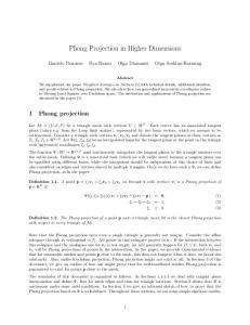
Trust region method • Multi-dim parabola method: define approximate quadratic function, but limit the step • Here Dk is trust region radius • Evaluate at previous iteration and compare the actual reduction to predicted reduction

• If rk around 1 we can increase Dk • If close to 0 or negative we shrink Dk

• Direction changes if Dk changes • If trust region covers p=0 step there

Line search vs trust region

1st order: gradient descent • We have a vector of parameters a and a scalar loss (cost) function J(a,x,y) which is a function of a data vector (x,y) we want to optimize (say minimize). This could be a nonlinear least square loss function: J=c2 • (Batch) gradient descent updates all the variables at once: da=-h▽a J(a): in ML h is called learning rate • It gets stuck on saddle points, where gradient is 0 everywhere (see animation later)

Scaling • Change variables to make surface more circular • Example: change of dimensions

Stochastic gradient descent

• Stochastic gradient descent: do this just for one data pair xi,yi: da=-h▽a J(a,xi,yi) • This saves on computational cost, but is noisy, so one repeats it by randomly choosing data i • Has large fluctuations in the cost function

• This is potentially a good thing: it may avoid getting stuck in the local minima (or saddle points) • Learning rate is slowly reduced • Has revolutionized machine learning

Mini-batch stochastic descent

• Mini-batch takes advantage of hardware and software implementations where a gradient wrt to a number of data points can be evaluated as fast as a single data (e.g. minibatch of N=256) • Challenges of (stochastic) gradient descent: how to choose learning rate (in 2nd order methods this is given by Hessian) • Ravines:

Ravines

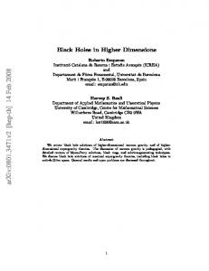
Adding momentum: rolling down the hill • We can add momentum and mimic a ball rolling down the hill • Use previous update as the direction • vt=gvt-1+h▽a J(a), da=-vt with g of order 1 (e.g. 0.9) • Momentum increases for directions where gradient does not change

Nesterov accelerated gradient • We can predict where to evaluate next gradient using previous velocity update • vt=gvt-1+h▽a J(a-gvt-1), da=-vt • Momentum (blue) vs NAG (brown+red=green)

• See https://arxiv.org/abs/1603.04245 for theoretical justification of NAG based on a Bregman divergence Lagrangian

Adagrad, adadelta, Rmsprop, ADAM… • Make the learning rate h dependent on ai • Use past gradient information to update h • Example ADAM: ADAptive Momentum estimation • mt=β1mt-1+(1−β1)gt gt=▽a J(a) • vt=β2vt-1+(1−β2)gt2 • bias correction: mt’=mt/(1-β1), vt’=vt/(1-β2) • Update rule: da=-h/(vt’1/2+e) • Recommended values b1=0.9, b2=0.999, e=10-8 • The methods are empirical (show animation)

nd 2

order methods: Newton

• We have seen that there is no natural way to choose learning rate in 1st order methods • But Newton’s method provides a clear answer what the learning rate should be: • J(a+da)=J(a)+da▽a J(a)+dada’ ▽a ▽a’ J(a)/2… • Hessian Hij= ▽a_i ▽a_j J(a) • At the extremum we we want ▽a J(a)=0 so a Newton update step is da=-H-1 ▽a J(a) • We do not need to guess the learning rate • We do need to evaluate Hessian and invert it (or use LU): expensive in many dimensions! • In many dimensions we use iterative schemes to solve this problem

Quasi-Newton • Computing Hessian and inverting it is expensive, but one can approximate it with a low rank tensor • Symmetric rank 1 (SR1) • BFGS (rank 2 update, positive definite) • Inverse (Woodburry formula)

L-BFGS • For large problems this gets too expensive. Limited memory BFGS updates only based on last N iterations (N of order 10-100) • In practice increasing N often does not improve the results • Historical note: quasi-Newton methods originate from W.C. Davidon’s work in 1950s, a physicist at Argonne national lab.

Linear conjugate direction • Is an iterative method to solve Ax=b (so belongs to linear algebra) • Can be used for optimization: min J=xTAx-bTx • Conjugate vectors: piApj=0 for all i,j not equal i • Construction similar to Gram-Schmidt (QR), where A plays the role of scalar product norm: xk+1=xk+akpk where ak=-rkTpk/(pkTApk) and rk=Axk-b • Essentially we are taking a dot product (with A norm) of the vector with previous vectors to project it perpendicular to previous vectors • Since the space is N-dim after N steps we have spanned the full space and converged to true solution, rN=0.

Conjugate direction • If we have the matrix A in diagonal form so that basis vectors are orthogonal we can find the minimum trivially along the axes, otherwise not

Linear conjugate gradient

• Computes pk from pk-1 • We want the step to be linear combination of residual –rk and previous direction pk-1 • pk=–rk +bkpk-1 premultiply by pTk-1A • bk= (rkApk-1)/(pTk-1Apk-1) imposing pTk-1Apk=0 • Converges rapidly for similar eigenvalues, not so much if condition number is high

Preconditioning • Tries to improve condition number of A by multiplying by another matrix C that is simple

• We wish to reduce condition number of • Example: incomplete Cholesky A=LLT by computing only a sparse L • Preconditioners are very problem specific

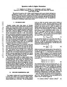
Nonlinear conjugate gradient • Replace ak with line search that minimizes J, and use xk+1=xk+akpk • Replace rk=Axk-b with gradient of J: ▽a J • This is Fletcher-Reeves version, Polak-Ribiere modifies b • CG is one of the most competitive methods, but requires the Hessian to have low condition number • Typically we do a few CG steps at each k, then move on to a new gradient evaluation

CG vs gradient descent In 2d CG has to converge in 2 steps

Gauss-Newton for nonlinear least squares

Line search in direction da

We drop 2nd term in Hessian because residual r=yi-y is small, fluctuates around 0 and because y’’ may be small (or zero for linear problems)

Gauss-Newton + trust region = Levenberg-Marquardt method • Solving ATAda=ATb is equivalent to minimize |Ada-b|2 • if trust region is within the solution just solve this equation • If not we need to impose ||da||=Dk • Lagrange multiplier minimization equivalent to (ATA+lI)da=ATb and l(D-||da||)=0 • For small l this is Gauss-Newton (use close to minimum), for large l this is steepest descent (use far from minimum) • A good method for nonlinear least squares

Literature • • • •

Numerical Recipes Ch. 9, 10, 15 Newman, Ch. 6 Nocedal and Wright, Optimization https://arxiv.org/abs/1609.04747