Phong Projection in Higher Dimensions

Phong Projection in Higher Dimensions Daniele Panozzo

Ilya Baran

Olga Diamanti

Olga Sorkine-Hornung

Abstract We supplement our paper Weighted Averages on Surfaces [1] with technical details, additional intuition, and proofs related to Phong projection. We also show how our generalized barycentric coordinates reduce to Moving Least Squares over Euclidean space. The motivation and applications of Phong projection are discussed in the paper [1].

1

Phong projection

Let M = (V, E, F) be a triangle mesh with vertices V ⊂ RD . Each vertex has an associated tangent plane (taken e.g. from the Loop limit surface), represented by two basis vectors, which we assume to be orthonormal. Consider a triangle with vertices v1 , v2 , v3 and denote the tangent planes at these vertices as T1 , T2 , T3 ∈ R2×D . Let Ψ(ξ1 , ξ2 , ξ3 ) be an interpolated basis for the tangent plane at the point on the triangle with barycentric coordinates ξ1 , ξ2 , ξ3 . The function Ψ : R3 → R2×D must continuously interpolate the tangent planes to the triangle interiors over the entire mesh. Defining Ψ is a non-trivial task (which we will tackle later) because a tangent plane can be specified using different bases, while the interpolant should be independent of this choice of basis and also consistent on edges and vertices shared by multiple triangles. Once we do have such a Ψ, we can define Phong projection, as in the paper: ˆ = ξ1 v1 + ξ2 v2 + ξ3 v3 on triangle t with vertices vi is a Phong projection of Definition 1.1. A point p p ∈ RD if: Ψ(ξ1 , ξ2 , ξ3 ) (ξ1 v1 + ξ2 v2 + ξ3 v3 − p) ξ1 + ξ2 + ξ3 ξi

= 0,

(1)

=

1,

(2)

≥ 0.

(3)

Definition 1.2. The Phong projection of a point p onto a triangle mesh M is the closest Phong projection with respect to every triangle of M. Note that the Phong projection onto even a single triangle is generally not unique. Consider the affine subspace through v1 orthogonal to T1 . All points in that subspace project to v1 . If the intersection between this subspace and the analogous one for v2 is not empty (as will generally happen for D ≥ 4), both v1 and v2 will be Phong projections of points in the intersection. In the paper, we provide experimental evidence that for reasonable meshes and points p close to the mesh, this does not happen; when it does, we break ties arbitrarily. Also, unlike Euclidean projection, Phong projection might not exist at all. In Section 3 of this document, we give an outline of how one might prove that for well-tessellated meshes Phong projection is guaranteed to exist for points p close to the mesh. The remainder of this document is organized as follows. In Sections 1.1-1.4 we deal with tangent plane interpolation and define Ψ, first for mesh edges and then for triangle interiors. Section 2 shows that Ψ is continuous under some mild conditions. In Section 3 we give an informal sketch of how to prove that the Phong projection based on Ψ is well-defined. Throughout these sections, we use some simple algebraic results;

1

we concentrate all these auxiliary propositions and their proofs in Section 4 in order to avoid clutter in the exposition. Finally, in Section 5 we show the equivalence between our generalized barycentric coordinates (see Section 3.4 in the paper) and Moving Least Squares when working in Euclidean spaces.

1.1

Plane representation

We now discuss how to work with planes in a D-dimensional space, each represented by a basis encoded in a 2-by-D matrix. Definition 1.3. Let T, K ∈ R2×D be two rank-2 matrices. If there exists a non-singular matrix A ∈ R2×2 for which K = AT , then T and K represent the same plane. We call such pairs of 2-by-D matrices equivalent and write T ≡ K. If T and K are equivalent and each has orthonormal rows, the matrix A relating them is orthogonal. Definition 1.4. For T ∈ R2×D , we denote by Ort(T ) the nearest orthonormal basis to T , i.e., Ort(T ) =

argmin

kT − Bk.

B∈R2×D : BB T =I

In the definition above and for the remainder of this document, the matrix norm k · k stands for the Frobenius norm, unless explicitly stated otherwise. Definition 1.5. If T and K both have rank 2, we measure the distance between the planes they represent as d(T, K) = min kOrt(T ) − A Ort(K)k. A∈O(2)

Letting T 0 = Ort(T ) and K 0 = Ort(K), we show in Proposition 4.4 that at the minimum, A = Ort(T 0 K 0T ) and that this distance is equivalent up to a constant to the more standard projection operator distance kT 0T T 0 − K 0T K 0 k (Propositions 4.6 and 4.7).

1.2

Interpolation requirements

The interpolation operator Ψ needs to satisfy some simple conditions for the interpolation to work. Given barycentric weights Ξ = (ξ1 , ξ2 , ξ3 ), where ξ1 + ξ2 + ξ3 = 1, ξi ≥ 0, we want to find a blended plane Ψ(ξ1 , ξ2 , ξ3 ) ∈ R2×D such that: Interpolation at vertices. Ψ(1, 0, 0) ≡ T1 , Ψ(0, 1, 0) ≡ T2 , Ψ(0, 0, 1) ≡ T3 . Interpolation at edges. For ξ1 , ξ2 ≥ 0, ξ3 = 0, Ψ(ξ1 , ξ2 , ξ3 ) does not depend on T3 or v3 (it depends only on T1 , T2 , v1 and v2 ). Same for the other two edges of the triangle and in general for each mesh edge. Continuity. While the basis interpolation Ψ(ξ1 , ξ2 , ξ3 ) does not have to be continuous, the corresponding planes do. Formally, continuity at Ξ is: ∀ > 0 : ∃δ : ∀Ξ0 : kΞ0 − Ξk < δ =⇒ d(Ψ(Ξ0 ), Ψ(Ξ)) < . The problem with defining Ψ(ξ1 , ξ2 , ξ3 ) = ξ1 T1 + ξ2 T2 + ξ3 T3 is that the blend depends on how the bases of the tangent planes are chosen (it may lead to results that belong to different equivalence classes) and can also lead to singularities. The goal is to fix this by choosing the bases intelligently. One cannot choose them globally due to hairy ball theorems, so the bases have to be different for every triangle. The difficulty then is keeping the blending consistent across edges. It is also possible to define a blend using the natural metric on the Grassmannian, but the resulting computations are complicated and expensive; we therefore choose to linearly blend bases. 2

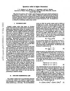
Figure 1: The planes at v1 and v2 are represented by two orthonormal bases T1 and T2 . The orthogonal matrix R12 transforms T1 in-plane, relative to T2 . Also, both bases T1 and T2 can be simultaneously rotated in-plane by the same orthogonal matrix E12 . R12 and E12 are degrees of freedom we can play with to optimize our tangent plane blending Ψ. We choose R12 such that it transforms T1 to be as close as possible to T2 and we also pick E12 to obtain a well-defined blend within the triangle, as described in Section 1.4.

1.3

Interpolation on edges

We construct Ψ in two steps: first, we define an interpolant on edges only, and then extend it to the interiors of the triangles. We start by defining the blends on the edges, i.e., when one of ξ1 , ξ2 , or ξ3 is zero. To have consistent interpolation between triangles that share an edge, we must carefully pick the bases to blend. Assume, without loss of generality, that ξ3 = 0. We then define Ψ as a blend between T1 and T2 as: Ψ(ξ1 , ξ2 , 0) = ξ1 R12 T1 + ξ2 R21 T2 ,

(4)

where R12 and R21 are orthonormal 2-by-2 matrices. Using R12 and R21 effectively allows us to pick bases for T1 and T2 (see Definition 1.3) that can be linearly blended without introducing singularities. Note that R12 and R21 are associated with an edge, so Ψ will behave consistently on both triangles that share that edge. We observe that having both R12 and R21 is redundant since: Observation 1.1. Let Ti for i = 1..n be bases (not necessarily orthonormal) for planes and let A ∈ R2×2 be a nonsingular matrix. Let ξi be scalar weights. Then we can multiply every Ti by A on the left without changing the plane: X X X ξi ATi = A ξi Ti ≡ ξi Ti . i

i

i

Corollary 1.1. If R1 , R2 ∈ R2×2 are orthogonal matrices and ξ1 , ξ2 > 0, ξ1 + ξ2 = 1 then ξ1 R1 T1 + ξ2 R2 T2 ≡ ξ1 R2T R1 T1 + ξ2 T2 . We can then assume without loss of generality that R21 = I and focus on choosing R12 . We choose it to minimize the difference between the bases (see Figure 1): R12 = Ort(T2 T1T ).

(5)

This choice is motivated by the fact that linearly interpolating bases that are close will always generate a valid basis. Proposition 4.3 shows that this choice is unique for sufficiently close planes, and then the blend on edges is independent of the bases chosen for the tangent planes. Definition 1.6. For ξ1 , ξ2 ≥ 0, ξ1 + ξ2 = 1, we choose the blend Ψ(ξ1 , ξ2 , 0) such that Ψ(ξ1 , ξ2 , 0) ≡ ξ1 Ort(T2 T1T ) T1 + ξ2 T2 . Proposition 1.1. The plane defined by Ψ(ξ1 , ξ2 , 0) does not depend on how T1 and T2 are chosen. 3

Proof. Recall that we assume that the tangent plane bases at vertices are always chosen to be orthonormal, hence it suffices to check that Ψ always remains in the same equivalence class when T1 and T2 are transformed by some in-plane rotations or reflections. Let X1 and X2 be arbitrary 2-by-2 orthogonal matrices. We have T1 ≡ X1 T1 , T2 ≡ X2 T2 . Let us check the blend (Definition 1.6) using these bases:

Cor. 1.1 ξ1 Ort (X2 T2 )(X1 T1 )T (X1 T1 ) + ξ2 (X2 T2 ) ≡ ξ1 X2T Ort X2 T2 T1T X1T X1 T1 + ξ2 T2 =

1.4

ξ1 X2T X2 Ort(T2 T1T )X1T X1 T1

+ ξ2 T2 =

ξ1 Ort(T2 T1T )T1

Prop. 4.1

=

+ ξ2 T2 ≡ Ψ(ξ1 , ξ2 , 0).

Interpolation on the triangle interior

So now we know how to blend along edges in a way that only depends on the tangent planes at the edge vertices. We need to extend the blend to the triangle interior in a continuous way. As before, let T1 , T2 , and T3 be the original orthonormal bases for the tangent planes at the triangle vertices. Let R12 = Ort(T2 T1T ),

R23 = Ort(T3 T2T ),

R31 = Ort(T1 T3T ).

such that Ψ(ξ1 , ξ2 , 0) ≡ ξ1 R12 T1 + ξ2 T2 , Ψ(0, ξ2 , ξ3 ) ≡ ξ2 R23 T2 + ξ3 T3 , Ψ(ξ1 , 0, ξ3 ) ≡ ξ3 R31 T3 + ξ1 T1 . To define the blend of all three tangent planes in the triangle interior, we extend each edge blend to the interior separately and then blend the three extensions using the weights 1/ξ1 , 1/ξ2 and 1/ξ3 (see Figure 2). To do this, we first need to blend each edge blend with the third tangent plane. For both this blend and the blend between the three extensions, the bases once again need to be consistent, or in other words, the result should not depend on the choice of the bases for T1 , T2 , T3 . Note that in Definition 1.6 we have a degree of freedom per edge in form of a transformation by an orthogonal matrix, i.e., we defined Ψ(ξ1 , ξ2 , 0) up to the equivalence class. Let us denote these degrees of freedom as orthogonal matrices E12 , E23 , E31 ∈ R2×2 for each edge (see Figure 1). Definition 1.7. Edge blend: Ψ(ξ1 , ξ2 , 0) = ξ1 E12 R12 T1 + ξ2 E12 T2 , where the choice of the orthogonal matrix E12 ∈ R2×2 will be explained below (in Definition 1.9). The definitions for the other edge blends are analogous.

v3

Ψ31

Ψ

Ψ23

v2

v1 Ψ12

Figure 2: We define a continuous blend for each pair of adjacent triangles (flaps) on the mesh (left). To compute Ψ over the black triangle, we blend the interpolants on the overlapping flaps using the weights 1/ξ1 , 1/ξ2 and 1/ξ3 (right).

4

Definition 1.8. Extension of a single edge blend to the triangle interior: 1 Ψ12 (ξ1 , ξ2 , ξ3 ) = ξ1 E12 R12 T1 + ξ2 E12 T2 + ξ3 (E23 + E31 R31 )T3 . 2 The definitions for Ψ23 and Ψ31 are similar. We choose the matrices E12 , E23 , E31 so that the matrices: E12 R12 T1 , E12 T2 , E23 R23 T2 , E23 T3 , E31 R31 T3 , E31 T1 are all as close to each other as possible, such that a linear blend between them would be non-singular. Definition 1.9. Denote A1 = E12 R12 T1 , A2 = E12 T2 , A3 = E23 R23 T2 , A4 = E23 T3 , A5 = E31 R31 T3 , A6 = E31 T1 . We choose the in-plane transformation per edge as follows: X E12 , E23 , E31 = argmin kAi − Aj k2 . (6) E12 ,E23 ,E31 ∈O(2) 1≤i