Lecture Notes in Computer Science - Muscle

Automatic Fuzzy-Neural based Segmentation of Microscopic Cell Images Sara Colantonio1, Igor B. Gurevich2, Ovidio Salvetti1 1

Istituto di Scienza e Tecnologie dell’Informazione, ISTI-CNR Via G. Moruzzi 1, 56124 Pisa, Italy {Sara.Colantonio,Ovidio.Salvetti}@isti.cnr.it http://www.isti.cnr.it/ResearchUnits/Labs/si-lab/ 2 Dorodnicyn Computing Centre of the Russian Academy of Sciences 40, Vavilov str., Moscow GSP-1 119991 The Russian Federation {igourevi}@ccas.ru

Abstract. In this paper, we propose a novel, completely automated method for the segmentation of lymphatic cell nuclei represented in microscopic specimen images. Actually, segmenting cell nuclei is the first, necessary step for developing an automated application for the early diagnostics of lymphatic system tumors. The proposed method follows a two-step approach to, firstly, find the nuclei and, then, to refine the segmentation by means of a neural model, able to localize the borders of each nucleus. Experimental results have shown the feasibility of the method.

1 Introduction A great deal of research has concerned, in the last years, the development of automated systems for the early diagnosis of lymphatic tumors based on the morphological analysis of blood cells in microscopic specimen images. Actually, pathologists usually make diagnosis by analyzing the morphology of specimen cells [1, 2]. The first and necessary step for automating cell analysis is an accurate segmentation of the cells themselves, which is, then, followed by the extraction of significant morphological parameters. Unfortunately, cell segmentation is usually an ill-posed problem: due to poor dye quality, cell boundary could be not well distinguishable and parts of the same tissue could be not equally stained; two or more cells could be very close to each other or even overlapping; the chromatin distribution inside the cells could generate strong computed edges which mislead the segmentation. In past years, many segmentation methods have been presented [3, 4]. They include watersheds [5, 6], region-based [7] and threshold-based methods [8]. The problem with these methods is that they do not employ any shape information of the cell, which can be useful in presence of noise. Recently, the application of Active Contours has been widely investigated for cell segmentation [9, 10]. However, such methods require an initialization of the snake,

making the segmentation not completely automated. Moreover, having to select which cell the snake should be apply to, much information regarding all the cells represented in the images is lost. Other contour-based methods include Active Shape Models (ASM) [11], Active Appearance Models (AAM) [12] and variational deformable models (Strings) [13]. In the first two cases, a boundary model and its allowed variations are learned from a set of example boundaries and represented by a set of labeled points, encoding only shape information in ASM, also image features in AAM. The Strings method differs from the previous ones in adopting a continuous instead of discrete boundary representation, together with a multiple features description, giving place to a multivariate curve representation in functional space (instead of a point representation in vector space). All these methods require initialization and allow modeling only the variation seen in the training set of boundary examples. The method we propose in this paper has the main characteristic to be completely automated. Moreover, it is suitable to segment all the cells contained in the images, allowing to extract information not only from the malignant ones. Following a two-step approach, images are first clustered, in order to perform a rough segmentation and localize the cells. In a second processing step, an Artificial Neural Network (ANN) is applied to the image portions containing the localized cell for individuating cell borders. Such an approach assures a high level of robustness, because the ANN performs a classification of the image and then it can distinguish among different kinds of structures, e.g. cell nucleus, cytoplasm, background, artifacts and so forth.

2 The Fuzzy-Neural Segmentation Microscopic cell images are acquired as footprints of lymphoid tissue stained according to the Romanovsky-Giemsa technique and digitized as color images. Each image I contains a number, say n, of cells which are constituted by the internal body – the nucleus –, which is the structure of interest to be segmented, and the cytoplasm. Due to the staining procedure, artifacts can be present in the images, as well as not perfectly stained cells that can be then considered as added noise. The proposed method is suitable to detect nuclei borders and consists in applying to each image I a two-stage procedure as follows: 1.

2.

Cell dislocation detection: a cluster analysis, based on the fuzzy c-means algorithm, is applied to identify and label homogeneous regions in the image. The clustered regions are then used to divide the entire image in disjoint sub-parts for further processing (image partition). Cells contours extraction: from each image partition relevant features are extracted and a dedicated ANN is used to complete the segmentation by identifying the contours of each cell.

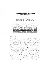
A sketch of the method is shown in Fig. 1.

Cells Dislocation Detection

Cells Contours Extraction

Cluster Analysis

Features Extraction

Image Partition

ANN for contour identification

Fig. 1. The two-step method for cell segmentation

In the following, each step is described in more details. 2.1 Cells Dislocation Detection In order to individuate how cells are dislocated in the microscopic images, a fuzzy cluster analysis is performed and each image is partitioned in disjoint parts for next step elaboration. Cluster Analysis. Homogeneous image regions are labelled using an unsupervised clustering method, based on the fuzzy c-means algorithm (FCM) [14]. This algorithm groups a set of data in a predefined number of classes so as to iteratively minimize a criterion function, namely the sum-of-squared-distance from region centroids, weighted by a cluster membership function. A membership grade p∈[0,1] is associated to each element of the data set, describing its probability to belong to a particular cluster. For each cell image I, a features vector (I0(x), I1(x), I2(x),…, Iq(x)) is computed for any pixel x, considering I(x) as a vector of the three color component I(x)=(r,g,b). Then I0(x) = I, and for k = 1,…,q, Ik(x) = I∗Γk(x), where Γk is a Gaussian filter with σ = k. In this way, we obtain a data set D = {v1, v2, …, vm} where each vh, h=1,…,m is a vector in ℜp representing image elements at different resolutions. Let Ucm be a set of real c × m matrices, with c being an integer, 2 ≤ c < m; the fuzzy c-partition space for D is, then, the set: c

m

i =1

h =1

Ω ={U ∈ U cm : uih ∈ [0,1], ∑ uik = 1,0 < ∑ uik < m} .

where uih is the membership value of vh in cluster i (i = 1,…,c).

(1)

By applying FCM, an optimal fuzzy c-partition and corresponding prototypes are found minimizing the objective function: m

c

Jη (U , Λ; D) = ∑∑ (uih )η v h − λ i h =1 i =1

2

.

(2)

where Λ = (λ1, λ2,…, λc) is a matrix of unknown cluster centers λi ∈ ℜp, ||⋅|| is any norm, e.g. the Euclidean norm, expressing the similarity between each data vector vh and the center λi, and the weighting exponent η ∈ [0,∞) is a constant that influences the membership values. Fuzzy partition is carried out through an iterative minimization of (2), calculating the cluster centers at each iteration t = 1,2,… as:

∑ ∑ m

λ i( t ) =

h =1 m

(uik(t ) )η v h

h =1

(uik( t ) )η

.

(3)

and updating the membership values as:

uik( t )

⎡ ⎢ c ⎛ v h − λ i( t ) = ⎢∑ ⎜ ⎢ j =1 ⎜ v h − λ (jt ) ⎝ ⎣⎢

−1

2 ⎤ ⎞η −1 ⎥ ⎟ ⎥ . 2 ⎟ ⎥ ⎠ ⎥ ⎦ 2

(4)

The iterative process stops when |U(t+1)-U(t)| follows under a certain threshold or the maximum number of iterations is reached. Applying the FCM on the cell images induces a partition of each slide into a set P={R1,R2,…} of disjoint connected regions R, where the indices 1,2,… are region labels. In other words, by clustering, we obtain a rough segmentation which can be refined reducing the computation by the following step of image partitioning. Image Partitioning. Once clustered the image, the convex hull of each connected region is calculated in order to delimitate the largest image portion (convex image) containing the corresponding connected region. Starting from the convex hull, an image partition is extracted slightly enlarged in both directions the convex image. Such partition contains what the FCM has classified as a unique cell. However, the contour of the clustered region can be inaccurate, including, for instance, the cytoplasm; moreover, it can happen that two very closed or touching cells are clustered as a unique region. For these reasons, it is necessary to refine the clusterization in a further step. 2.2 Cells Contour Extraction In order to detect the exact cell contour, from each image partition, a set of features is extracted and classified by a dedicated ANN.

Features Extraction. Analyzing the properties of cell images and of the similar cells, the following vector of features ℑ(x) is computed for characterizing each pixel x of the segmented image partition: ƒ ƒ

ƒ

ƒ

ƒ

Color values: I(x) = (r,g,b); Mean color value: M(x) = (Mr, Mg, Mb) computed applying an average filter F(x), i.e. M(x) = I(x) ∗F(x); Gradient norm: ||∇I(x)|| and its mean, computed along the three color components; Radial gradient: Grt(x), defined as the gradient component in the radial direction rˆ from the center of the connected region; Membership value to the clustered region: ui(x), where i is the cluster index considered as a cell in the image partition.

ANN for contours identification. The vectors of the extracted features ℑ(x) are processed by a dedicated ANN. It consists in a Multilayer Perceptron, trained according to the Error Back-Propagation (EBP) algorithm [15] to recognize five different classes. At present, to resolve ambiguity in case of touching cells and let the network learn and generalize better, five pixel classes are selected: 1. Cell border 2. Cell internal body 3. Cytoplasm 4. Background 5. Artifact Let oj(ℑ(x)) be the answer of the output units of the network when the features vector ℑ(x) is being processed; then, the pixel membership to one of the above mentioned classes can be computed as

Φ(x) = argmaxj=1,…,5(oj(ℑ(x))) .

(5)

A set of pre-classified images has been used to train the network, using the Resilient Back-Propagation [16] version of the EBP algorithm. Once defined the desired ψp output for each input vector of the training set TS = {ℑp(x)}, the cost function E=

1 |TS | ∑ (ψ p − o p )2 . 2 p =1

(6)

where op = (o1,o2,…,oj) is the output vector of the network, is minimized iteratively computing the weight update at each iteration step t as follows: ⎧ (t ) ⎪−∆ ij ⎪ ⎪⎪ ∆wij( t ) =⎨−∆ ij( t ) ⎪ ⎪0 ⎪ ⎪⎩

if

∂E (t ) > 0 ∂wij

if

∂E (t ) > 0 . ∂wij

otherwise

(7)

where wij is the weight between the network units i and j, and ∆ij is the amount of weight change which, starting from a chosen value ∆0, varies at each step t according to the following equation:

∆ (ijt )

⎧ + ( t −1) ⎪ε ∆ ij ⎪ ⎪⎪ = ⎨ε − ∆ (ijt −1) ⎪ ⎪ ( t −1) ⎪ ∆ ij ⎪⎩

if

∂E ∂E (t − 1) ⋅ (t ) > 0 ∂w ij ∂w ij

if

∂E ∂E (t − 1) ⋅ (t ) < 0 . ∂w ij ∂w ij

(7)

otherwise

where 0 < ε- < 1 < ε+ are parameters used to regulate weight modifications. The final result of this step is discussed in the following section.

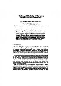
3 Results Footprints of lymphoid tissues were Romanovsky-Giemsa stained and digitized with digital camera mounted on Leica DMRB microscope using PlanApo 100/1.3 objective. The equivalent size of a pixel was 0,0036 µ2; 24-bit color images were stored in TIFF format of dimensions 1200 × 1792. A total number of 800 microscopic images were considered, with an average number of 20 cells for each. An example of a microscopic cell image and its three color components is reported in Fig. 2. The cluster analysis was designed to be performed on the features vectors (I0(x), I1(x), I2(x),…, Iq(x)) with q = 5, but, among such components, only I3(x) and I5(x) were considered relevant. The input vectors represented in the form of color images are shown in Fig. 3.

Original

Red Component

Green Component

Blue Component

Fig. 2. An example of microscopic cell image: the original image and the three color components.

Fig. 3. An example of the three-component feature vector used for clustering: from left to right, original, σ = 3 and σ = 5.

The same feature vector for each of the color components of the image is reported in Fig. 4. The FCM algorithm is applied to divide image pixels into two clusters corresponding to cell and background. A filling operation is performed to eliminate little holes, while clustered regions of negligible area are deleted. An example of the clustering results is reported in Fig. 5.

Red component

original Green component

σ=3

σ=5

original Green component

σ=3

σ=5

original

σ=3

σ=5

Fig. 4. An example of the feature vector with the original values I0(x) and I3(x) and I5(x) for each of the three color components.

Fig. 5. Example of the clustering results: rough clustered image (left), clustered image after a filling operation and after deletion of regions of negligible area (right).

Examples of image partitions extracted for detecting the exact borders of a cell are shown in Fig. 6.

Fig. 6. Image partitions containing the cells to be segmented.

From each partition, the set of the mentioned features is extracted. To illustrate the significance of such set, Fig. 7 shows an example of the gradient regarding the green component. The set of 800 images was partitioned in (i) a sub-set of 300 images, used for training, and (ii) a sub-set of the remaining 500 images used for the testing phase. A semiautomatic segmentation was performed for the training set, consisting in a classification of images according to the different classes of pixels. Different architectures were tested, varying the number of the hidden units: the best performance was achieved with only one hidden layer of 20 units. An example of the segmentation results is illustrated in Fig. 8, where the entire classification results are reported too.

Fig. 7. Example of the computation of the green component gradient along the horizontal axis (left), along the vertical axis (middle) and the norm of the same gradient (right).

4 Discussion and Conclusions A two-step method for segmenting microscopic cell images has been presented.

The first step consists of a fuzzy clustering of images performed to obtain a rough segmentation and to detect cell dislocation. In the second step, a dedicated ANN is applied to refine the segmentation by discriminating image components, i.e. cell borders, cell internal body, cytoplasm, background, and artifacts. The main features of the proposed method are ƒ complete automation of segmentation ƒ possibility of extracting all the cells represented in the images ƒ robustness due to the ANN application which allows resolving ambiguity of closed or touching cells. An example of the last characteristic is shown in Fig. 9, where it can be seen how two cells that are clustered as a unique region by the FCM are well separated by the ANN thanks to the individuation of cytoplasm.

Original

ANN classification Cell internal body Cell contour Cytoplasm Background Artifact

Contour Extracted

Fig. 8. Example of segmentation. upper left: original cell image; upper right: results of the ANN classification (five classes with different colors); lower left: identified contours of each cell; lower right, legenda.

Fig. 9. Example showing the robustness of the proposed method: (left) rough segmentation obtained by FCM that individuates a unique region corresponding to three different cells; (right) result of the ANN algorithm where the cells are correctly separated by classifying pixels in cell body, cytoplasm and artifact (see Fig. 8 for explanation of colors).

Acknowledgment This work was partially supported by INTAS Grant N 04-77-7067, by the Cooperative grant “Image Analysis and Synthesis: Theoretical Foundations and Prototypical Applications in Medial Imaging” within bilateral agreement between Italian National Research Council and Russian Academy of Sciences, by European Project Network of Excellence MUSCLE – FP6-507752 (Multimedia Understanding through Semantics, Computation and Learning), and by the Russian Foundation for Basic Research Grant N 05-07-08000.

References 1. Zh.V. Churakova, I.B. Gurevich, I.A. Jernova, et al. Selection of Diagnostically Valuable Features for Morphological Analysis of Blood Cells, Pattern Recognition and Image Analysis: Advances in Mathematical Theory and Applications, Vol. 13. (2003) 2 381-383 2. Jaffe E. S , Harris N. L., Stein H., et al. Pathology and Genetics of Tumors of Haematopoietic and Lymphoid Tissues. Lyon: IARC Press (2001) 3. Di Rubeto, C., Dempster, A., Khan S., Jarra, B.: Segmentation of Blood Image using Morphological Operators. Proc. 15th Int. Conference on Pattern Recognition (2000), 3 397-400 4. Anoraganingrum, D.: Cell Segmentation with Median Filter and Mathematical Morphology Operation. Proceeding International Conference on Image Analysis and Processing (1999), 1043-1046 5. Lin G., Adiga U., Olson K., Guzowski J.F., Barnes CA, Roysam B.: A hybrid 3D watershed algorithm incorporating gradient cues and object models for automatic segmentation of nuclei in confocal image stacks. Cytometry A. (2003), 56, 1, 23-36

6. Umesh Adiga P.S. and Chaudhuri B.B., “An efficient method based on watershed and rulebased merging for segmentation of 3-D histopathological images. Pattern Recognition (2001), 34, 7, 1449-1458 7. Mouroutis, T., Roberts, SJ., Bharath. AA.: Robust cell nuclei segmentation using statistical modelling. BioImaging (1998), 6, 79-91 8. Wu, HS., Barba, J., Gil, J.: Iterative thresholding for segmentation of cells from noisy images. J. Microsc. (2000), 197,296-304 9. Karlosson, A., Strahlen, K., Heyden, A.: Segmentation of histological section using snakes. In J. Begun and T. Gustavsson, eds. LNCS 2749, Proc. of 13 Scandinavian Conference, SCIA 2003, Halmstad, Sweeden (2003), 595-602 10. Murashov, D.: Two-level method for segmentation of cytological images using active contour model. Proc. 7th Int. Conference on Pattern Recognition and Image Analysis, PRIA -7 (2004), III, 814-817 11. Cootes T.F. and Taylor C.J.: Active Shape Models – ‘Smart Snakes’, Proc. British Mach. Vision Conf., Springer-Verlag (1992), 266-275 12. Cootes T. F., Beeston C., Edwards G. J., Taylor C. J.: A unified framework for atlas matching using active appearance models, in Information Processing in Medical Imaging, A. Kuba and M. Samal, Eds. Berlin, Germany: Springer-Verlag, Lecture Notes in Computer Science (1999), 322–333. 13. Ghebreab S. and Smeulders A.W.M.: Strings: Variational Deformable Models of Multivariate Continuous Boundary Features, IEEE Transactions on Pattern Analysis And Machine Intelligence (2003), 25, 11, 1399-1410 14. Bezdek, L.C.: Pattern Recognition with Fuzzy Objective Function Algorithm, New York: Plenum Press, 1981 15. Rumelhart, DE., Hinton, GE., Williams, RJ.: Learning internal representations by error propagation” Parallel Distribuited Processing (1986) MIT Press, Cambridge, MA, 318-362. 16. Riedmiller, M., Braun, H.: A direct adaptive method for faster backpropagation learning: The RPROP algorithm. Proc. of the IEEE International Conference on Neural Networks – ICNN, (1993), 586-591