Lecture Notes on Data Science: Principal. Component ... This is the first in a series of lecture notes on principal component .... J. of Educational Psychology, 24.
Lecture Notes on Data Science: Principal Component Analysis (Part 1) Christian Bauckhage B-IT, University of Bonn This is the first in a series of lecture notes on principal component analysis (PCA) and its applications in data science. We begin our study by looking at two of the fundamental use cases for this method.
Introduction
e2
It is hardly exaggerated to claim that principal component analysis, or PCA for short, is one of the most important tools of the trade in data science. In fact, it is of fundamental importance for scientific computing in general. In this series of lectures, we will therefore acquaint ourselves with its foundations, properties, and applications. In order to motivate us for the things to come, we will begin our study by looking at two important applications of the method.
e1
(a) 2D data sample
u2
Data Decorrelation Figure 1(a) shows a sample of 2D data points plotted in a Cartesian coordinates system spanned by two basis vectors e1 and e2 . Looking at this example, it appears as if the variables expressed by the e1 , e2 coordinates of these data points are correlated. To better understand the notion of correlation, let us assume we were a tiny ant walking along the axis indicated by e1 . Looking up at the data points, it would appear to us that, the further we walk, the higher up the data will be (at least on average). That is, we would notice a trend: data points with small e1 -coordinates tend to also have small e2 -coordinates while data points with larger e1 coordinates seem to have larger e1 -coordinates. Hence, seen over the whole sample, point coordinates are not independent but correlated. However, this may be an artifact of our point of view. Figure 1(b) shows another Cartesian coordinate system whose origin and basis vectors differ from the one we considered above. If we were to change our point of view and would express the data in terms of their u1 , u2 -coordinates (see Fig. 1), we would not find any noticeable correlation. That is, a tiny ant walking along the axis indicated by u1 would not conclude that small or large u1 -coordinates imply small or large u2 -coordinates. In other words, in the u1 , u2 system, the data are de-cdorrelated. Since de-correlated data are a prerequisite for many data mining and pattern recognition algorithms, this begs the obvious question of how to determine a coordinate system such as in Fig. 1(b)? And the arguably most popular answer is (of course): using principal component analysis!
u1 e2
e1
(b) principal axes
u2
e2
u1
e1 (c) change of coordinates Figure 1: Linear decorrelation via PCA.
lecture notes on data science: principal component analysis (part 1)
2
Dimensionality Reduction and Data Compression In practice, we are often confronted with very high dimensional data points which pose fundamental difficulties for data analysis1 . Of course, for our exemplary data set of 2D data points in Fig. 1, we will not encounter any of these problems but it allows us to exemplify how to address them. A possible idea for dealing with high dimensional data consists in analyzing if all the measurements expressed by a data point really contribute to the solution of the analytics problem at hand or if some of them can be ignored. Mathematically, the simplest way of reducing the dimensionality of a data data point is to project it into a lower dimensional space. This is illustrated in Fig. 2(a) which shows a simple orthogonal projection from 2D to 1D. Alas, looking at the projected one-dimensional data points, it appears as if they severely overlap. That is to say, while the original 2D points are rather well distinguishable, the naïve strategy of “throwing away” e1 -coordinates leads to a situation where points that were different become similar. Well, what if we instead “throw away” all the e2 coordinates and keep the e1 values of the data points? Figure 2(b) shows that, at least for our current example, this seems to be a better idea. Here, the 1D representations of the originally 2D points do not overlap quite so severely. Yet, there still is overlap and, in general, i.e. in really high dimensional settings, it is of course not at all clear which and how many dimensions of our data to ignore. A principled approach and criterion would be well appreciated.
This is because of the so called curse of dimensionality which we will discuss in another note.
1
(a) projection onto axis along e2
Again, principal component analysis comes to the rescue. In Fig. 2(c), we see a projection of our 2D data onto the u1 axis of the coordinate system discussed above. Of course, we again loose information which is to say that the resulting lower dimensional data points are again less distinguishable than the original higher dimensional ones. But, we can (and will) indeed prove mathematically that, among all techniques based on linear projections, principal component analysis is the linear dimensionality reduction technique that best preserves information. Moreover, we can (and will) show that principal component analysis provides a systematic criterion for deciding how many dimensions to keep.
(b) projection onto axis along e1
Finally, we note that dimensionality reduction can also be understood as data compression. By projecting the 100 data points in our example from the two-dimensional space R2 into a one-dimensional subspace R, we reduced the amount of data to be stored from 2 × 100 (floating point) numbers to 100 (floating point) numbers. Hence, if there are reasons for us to opt for linear data compression techniques, PCA will again be the method of choice.
(c) projection onto axis along u1 Figure 2: Linear dimensionality reduction via principal component analysis.
lecture notes on data science: principal component analysis (part 1)
3
Notes and References Principal component analysis has a venerable history and numerous applications all across the sciences. Just as many techniques (from the pre-Internet age) it has been independently developed by several researchers. The earliest modern reference seems to consist in work by Pearson in 19012 and its now so commonly used name appears to be due to Hotelling3 . At the same time, the method is also frequently referred to as the Karhunen-Loève transformation4 . Famous application examples in the context of pattern recognition can be found in computer vision where PCA applies to real- and complex-valued data, alike5 , 6 . PCA also plays a key role in spectral clustering 7 , 8 and therefore provides an approach to graph clustering and network partitioning9 .
K. Pearson. On Lines and Planes of Closest Fit to Systems of Points in Space. Philosophical Magazine, 2(11), 1901 3 H. Hotelling. Analysis of a Complex of Statistical Variables into Principal Components. J. of Educational Psychology, 24 (7), 1933 4 K. Karhunen. Über lineare Methoden in der Wahrscheinlichkeitsrechnung. Ann. Acad. Scientiarum Fennicæ: Mathematika – Physica, 37, 1947 2
L. Sirovich and M. Kirby. Lowdimensional Procedure for the Characterization of Human Faces. J. Optical Society of America A, 4(3), 1987 5
C. Bauckhage and J.K. Tsotsos. Image Space I3 and Eigen Curvature for Illumination Insensitive Face Detection. In Proc. ICIAR, 2005 7 M. Fiedler. A Property of Eigenvectors of Nonnegative Symmetric Matrices and its Application to Graph Theory. Czechoslovak Mathematical J., 25(4), 1975 8 U. von Luxburg. A Tutorial on Spectral Clustering. arXiv:0711.0189, 2007 6
C. Bauckhage, R. Sifa, A. Drachen, C. Thurau, and F. Hadiji. Beyond Heatmaps: Spatio-Temporal Clustering using Behavior-Based Partitioning of Game Levels. In Proc. CIG, 2014 9
lecture notes on data science: principal component analysis (part 1)
References [1] C. Bauckhage and J.K. Tsotsos. Image Space I3 and Eigen Curvature for Illumination Insensitive Face Detection. In Proc. ICIAR, 2005. [2] C. Bauckhage, R. Sifa, A. Drachen, C. Thurau, and F. Hadiji. Beyond Heatmaps: Spatio-Temporal Clustering using BehaviorBased Partitioning of Game Levels. In Proc. CIG, 2014. [3] M. Fiedler. A Property of Eigenvectors of Nonnegative Symmetric Matrices and its Application to Graph Theory. Czechoslovak Mathematical J., 25(4), 1975. [4] H. Hotelling. Analysis of a Complex of Statistical Variables into Principal Components. J. of Educational Psychology, 24(7), 1933. [5] K. Karhunen. Über lineare Methoden in der Wahrscheinlichkeitsrechnung. Ann. Acad. Scientiarum Fennicæ: Mathematika – Physica, 37, 1947. [6] K. Pearson. On Lines and Planes of Closest Fit to Systems of Points in Space. Philosophical Magazine, 2(11), 1901. [7] L. Sirovich and M. Kirby. Low-dimensional Procedure for the Characterization of Human Faces. J. Optical Society of America A, 4(3), 1987. [8] U. von Luxburg. arXiv:0711.0189, 2007.
A Tutorial on Spectral Clustering.
4