Efficient saliency detection using regional color and spatial ... - HAL-Inria

Efficient saliency detection using regional color and spatial information Shuhua Luo, Zhi Liu, Li Lina, Xuemei Zou, Olivier Le Meur

To cite this version: Shuhua Luo, Zhi Liu, Li Lina, Xuemei Zou, Olivier Le Meur. Efficient saliency detection using regional color and spatial information. EUVIP, Jun 2013, Paris, France. 2013.

HAL Id: hal-00876192 https://hal.inria.fr/hal-00876192 Submitted on 24 Oct 2013

HAL is a multi-disciplinary open access archive for the deposit and dissemination of scientific research documents, whether they are published or not. The documents may come from teaching and research institutions in France or abroad, or from public or private research centers.

L’archive ouverte pluridisciplinaire HAL, est destin´ee au d´epˆot et `a la diffusion de documents scientifiques de niveau recherche, publi´es ou non, ´emanant des ´etablissements d’enseignement et de recherche fran¸cais ou ´etrangers, des laboratoires publics ou priv´es.

EFFICIENT SALIENCY DETECTION USING REGIONAL COLOR AND SPATIAL INFORMATION Shuhua Luo1, Zhi Liu1,2, Lina Li1, Xuemei Zou1, and Olivier Le Meur2,3 1

School of Communication and Information Engineering, Shanghai University, Shanghai 200072, China 2 IRISA, Campus Universitaire de Beaulieu, Rennes 35042, France 3 University of Rennes 1, Campus Universitaire de Beaulieu, Rennes 35042, France

ABSTRACT In this paper, we propose an efficient saliency model using regional color and spatial information. The original image is first segmented into a set of regions using a superpixel segmentation algorithm. For each region, its color saliency is evaluated based on the color similarity measures with other regions, and its spatial saliency is evaluated based on its color distribution and spatial position. The final saliency map is generated by combining color saliency measures and spatial saliency measures of regions. Experimental results on a public dataset containing 1000 images demonstrate that our computationally efficient saliency model outperforms the other six state-of-the-art models on saliency detection performance. Index Terms—Saliency detection, saliency model, color saliency, spatial saliency. 1. INTRODUCTION Saliency detection plays an important role in many content-based applications such as salient object detection [1-2], salient object segmentation [3-5], content-aware image retargeting [6-8], content-based image retrieval [9] and content-based image/video compression [10], etc. A number of saliency models have been proposed in the past decades. In general, the output of saliency model is the saliency map, in which the pixels/regions attracting human visual attention are highlighted while background regions are suppressed. The saliency model proposed by Itti et al. [11] is motivated by simulating human visual attention mechanism. Itti’s model adopts the center-surround scheme that the salient pixels/regions should be distinguished from its surrounding pixels/regions, to calculate feature maps of luminance, color and orientation over different scales, and then performs normalization and summation operations to generate the saliency map. From then on, the center-surround scheme has been implemented using local contrasts of color, texture and shape features [12], multi-scale contrast and centersurround histogram [1], and Kullback-Leibler divergence between histograms of filter responses [13]. Besides, some extensions with the introduction of global

information are proposed in the recent center-surround scheme based saliency models. For example, the whole region of the blurred image is used as the surrounding region in the frequency-tuned saliency model [14], and the global uniqueness of color feature is exploited in the context-aware saliency model [15]. In [16], both local and global color difference at region level are used for measuring saliency. In [17], histogram/region based global contrast measures are evaluated with respect to all the other pixels/regions. Recently, the use of earth mover’s distance (EMD) is found useful for measuring the centersurround difference [18]. Besides the center-surround scheme, there are also other formulations for measuring saliency. Some saliency models are built using the features in the frequency domain, such as the spectrum residual of Fourier transform [19] and the phase spectrum of quaternion Fourier transform [10], to generate block-level saliency maps. Based on supervised learning, conditional random field is exploited in [1] to generate saliency maps and detect salient objects. Recently, different statistical models are efficiently utilized in saliency models to improve the quality of saliency map. Gaussian models [20] and kernel density estimation based nonparametric models [21], which are constructed for each segmented region, are exploited to derive the pixel-level saliency map. In [22], both orientation distribution and global color distribution, which is represented using Gaussian mixture models, are fully exploited to selectively generate the saliency map. In [23], color compactness measures of over-segmented regions are exploited to generate saliency map with welldefined boundaries. It should be noted that some saliency models such as [10-13, 18-19] generally generate spotlight saliency maps, which are more suitable for prediction of eye fixations. In contrast, other saliency models mentioned above can highlight the complete salient object regions better in the generated saliency maps, which are more suitable for content-based applications such as salient object detection and segmentation. In this paper, we propose an efficient saliency model, which effectively utilizes both color and spatial information at region level. The proposed saliency model performs well on highlighting salient regions and suppressing non-salient background regions, and can be effectively used for content-based applications. Compared

with the current state-of-the-art saliency models, the proposed model achieves an overall better saliency detection performance and computational efficiency. The rest of this paper is organized as follows. In Section 2, the proposed saliency model is described in detail. Experimental results are shown in Section 3, and conclusions are given in Section 4. 2. PROPOSED SALIENCY MODEL 2.1. Image segmentation

(a)

(b)

(c)

(d)

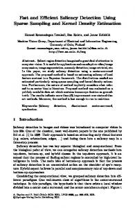
Fig. 1. (a) Superpixel segmentation result; (b) color saliency map; (c) spatial saliency map; (d) final saliency map.

shown using Fig. 1(b), in which brighter regions have higher color saliency values. We can observe from Fig. 1(b) that a majority of background regions are sufficiently suppressed, and different parts of the two persons are uniformly highlighted.

The input image is first segmented into a cluster of regions using the SLIC algorithm [24], which can result in an edge-preserving superpixel segmentation result. The two parameters in SLIC are set as follows. The spatial regularity parameter J is set to 0.5, and the number of superpixels D is set to 300, which can sufficiently preserve the boundaries of objects and structures without under-segmentation errors in natural images. Fig. 1(a) shows an example of superpixel segmentation result, in which boundaries between different regions are delineated using white lines. As shown in Fig. 1(a), superpixel segmentation generates regular-sized regions with better boundary adherence, and fits well for saliency evaluation at region level. Each segmented region Ri (i 1,!, n ) is used as the processing unit in the proposed saliency model. For each segmented region, its color saliency is evaluated based on the color similarity with all the other regions, and its spatial saliency is evaluated based on the color distribution and spatial position. The following two subsections will detail the proposed two measures, i.e., color saliency and spatial saliency, respectively.

Besides color similarity, the spatial distribution of color information and the factor of spatial position also contribute to the detection of salient objects in natural images. Based on the center-surround scheme, which has been widely implemented using different formulations in previous saliency models, salient objects are generally surrounded by non-salient background regions that usually scatter over the whole image. Therefore, the colors of background regions usually spread more widely over the whole image than the colors of salient regions, which usually distribute compactly. In addition, salient regions near to the image center are more likely to catch observer’s attention. Based on the above considerations, the spatial saliency of each region Ri is defined as

2.2. Color saliency

where d j denotes the ratio of Euclidean distance between

For each region Ri , its color similarity with all the other regions is defined as n  Di , j (1) exp( ) Ci ¦ aj j 1, j z i where a j is the area of region R j , and Di , j denotes the Euclidean distance on the mean color between Ri and R j in the Lab color space. Eq. (1) indicates that the regions whose colors are different from most of other regions in the image are assigned with a smaller value of color similarity, and the exponential form in Eq. (1) is used to reasonably magnify the color difference in the color similarity measure. Then the color similarity measures of all regions, Ci (i 1,!, n ) , are normalized into the range of [0, 1], and the color saliency of Ri is defined as

SiCol 1  Ci (2) Therefore, higher color saliency values are assigned to those regions that show higher color dissimilarity with most of other regions, and regions with similar colors have similar values of color saliency. For the example in Fig. 1(a), the color saliency values of all regions are

2.3. Spatial saliency

n

¦

SiSpa

j 1, j z i

exp(1  d j ) ˜ w(i, j )  exp(1  d i )

n

¦

(3)

w (i , j )

j 1, j z i

the centroid of R j and the image center to a half of the image diagonal length. The weight w(i, j ) is defined as w (i , j )

1 Di , j  H

(4)

where the constant H is set to a small value, 0.001, to avoid dividing by zero when Ri and R j share exactly the same mean color. Eq. (3) enables the region with a more compact color distribution to obtain a higher spatial saliency value, and reasonably promotes the spatial saliency values of regions that are nearer to the image center. Similarly as Fig. 1(b), the spatial saliency values of all regions are shown using Fig. 1(c). We can observe from Fig. 1(c) that those regions belonging to the two persons are highlighted, and background regions are gradually suppressed. 2.4. Saliency map generation

By integrating the above defined region-level color saliency and spatial saliency, the final saliency for each region Ri is defined as

(a) (b) (c) (d) Fig. 2. More examples of saliency map generation. (a) Original images; (b) color saliency maps; (c) spatial saliency maps; (d) final saliency maps.

Sali SiCol ˜ SiSpa (5) Eq. (5) indicates that the regions, which are salient in terms of both color saliency and spatial saliency, will achieve higher values of final saliency. The final saliency map for the example image in Fig. 1(a) is shown in Fig. 1(d), which is normalized into the range of [0, 255] for display. Compared with Fig. 1(b) and (c), we can see that background regions are more effectively suppressed in Fig. 1(d). We found from a variety of images such as those shown in Fig. 2 that color saliency and spatial saliency of regions can complement each other. Therefore, the finally generated saliency maps not only highlight salient regions, but also suppress background regions effectively. An objective evaluation on the effectiveness of integrating color saliency with spatial saliency will be presented in the following experimental results. 3. EXPERIMENTAL RESULTS

In order to evaluate the saliency detection performance, the proposed saliency model is experimented on a public image dataset [14], which contains the manually segmented binary salient object masks for 1000 images (available at http://ivrg.epfl.ch/supplementary _material/RK_CVPR09/index.html). These 1000 images are selected from Microsoft Research Asia Salient Object Database (MSRA SOD) Image Set B [1]. We generated the color/spatial/final saliency maps for all 1000 test images using the proposed saliency model. We adopted the commonly used precision and recall measures, and plot the precision-recall curves of the three classes of saliency maps to demonstrate the effectiveness of integrating color saliency with spatial saliency. Each saliency map is normalized into the same range of [0,255], and then we vary the integer threshold from 0 to 255 to obtain 256 binary salient object masks. Assume that each binary salient object mask is denoted by S , and the corresponding ground truth is denoted by G . In both S and G , each salient object pixel is labeled as “1”, and each background pixel is labeled as “0”. The precision and recall are defined as ¦ ( x , y ) S ( x, y ) ˜ G ( x, y ) (6) precision ¦ ( x , y ) S ( x, y )

Fig. 3. Precision-recall curves generated using our color saliency maps, spatial saliency maps and final saliency maps.

recall

¦

( x, y )

S ( x, y ) ˜ G ( x, y )

¦

( x, y )

G ( x, y )

(7)

For each class of saliency maps, at each threshold, the precision and recall measures calculated for all 1000 images are averaged, and the corresponding precisionrecall curve plots the 256 average precision values versus the 256 average recall values. We can observe from the three precision-recall curves in Fig. 3 that an obvious higher saliency detection performance is achieved by final saliency maps compared to both color and spatial saliency maps. We compared our saliency model against six state-ofthe-art saliency models including Itti’s (IT) model [11], spectral residual (SR) model [19], context-aware (CA) model [15], kernel density estimation (KD) based model [21], region contrast (RC) based model [17] and oversegmentation (OS) based model [23]. We used the implementation code of Saliency Toolbox [25] for IT model, and the authors’ executables or source codes with default parameter settings for the other five saliency models. For a fair comparison, all saliency maps are upsampled to the full resolution of original images and normalized into the same range of [0, 255]. A sample of saliency maps generated using our saliency model and the other six saliency models are shown in Fig. 4. Compared with the saliency maps generated using other saliency models, it can be seen from Fig. 4 that the saliency maps generated using our saliency model show a better performance on completely highlighting salient objects and effectively suppressing background regions. In order to objectively evaluate the saliency detection performance of different saliency models, similarly as Fig. 3, the precision-recall curves of all saliency models are shown in Fig. 5. We can see from Fig. 5 that precisionrecall curves of IT and SR, which are more suitable for prediction of eye fixation, are obviously lower than precision-recall curves of other saliency models. These precision-recall curves effectively demonstrate that our saliency model outperforms the other six saliency models on saliency detection performance.

(a) (b) (c) (d) (e) (f) (g) (h) (i) Fig. 4. Comparison of saliency maps generated for some test images. (a) Original images; (b) ground truths; (c)-(h) saliency maps generated using IT, SR, CA, KD, RC and OS, respectively; (i) our saliency maps.

In order to evaluate the suitability of saliency maps for salient object detection and segmentation in a straightforward way, we performed an adaptive thresholding operation [26] on each saliency map to obtain the binary salient object mask. The precision and recall are calculated for each saliency map by comparing the obtained binary salient object mask to the ground truth, and the F-measure, as a harmonic mean of precision and recall, is defined as

(1  E ) ˜ precision ˜ recall (8) E ˜ precision  recall where the coefficient E is set to 0.3 to weigh precision more than recall. For each saliency model, the average of precision, recall and F-measure on all 1000 saliency maps are calculated and shown in Fig. 6. We can see that the average F-measure of the proposed saliency model is higher than the other six models. Therefore, we can conclude that the quality of our saliency maps is generally F - measure

Fig. 5. Precision-recall curves of different saliency models.

Fig. 6. Average precision, recall and F-measure of different saliency models.

(a) (b) (c) (d) (e) (f) (g) (h) (i) Fig. 7. Failure cases. (a) Original images; (b) ground truths; (c)-(h) saliency maps generated using IT, SR, CA, KD, RC and OS, respectively; (i) our saliency maps.

better than saliency maps generated using the other six models for salient object detection and segmentation. However, there are some failure cases using our saliency model. As shown in Fig. 7, the color difference between the object and background regions is small in the top example, and the colors of some defocused regions are rare and distinctive in the bottom example. Since the color is an important factor in our saliency model, it is difficult for our model to effectively highlight salient regions in such cases. However, it can be seen from Fig. 7 that other saliency models also cannot handle such examples effectively. Besides, we also compared the average running time per image of our saliency model and several saliency models that show a better saliency detection performance in Fig. 5. We run all saliency models on a desktop PC with Intel Core i7-2600 3.4 GHz CPU and 4GB RAM. As shown in Table I, our saliency model is the most efficient one among the saliency models implemented using Matlab, and we believe that the computational efficiency of our model could be comparable to RC if our model is implemented using C++ with code optimization. Although the saliency detection performance of KD is very close to our saliency model as shown in Fig. 5, it can be seen from Table I that our model is almost 30 times faster than KD. It should be noted that the most time-consuming part of our saliency model is superpixel segmentation, which spends about 60% processing time. Further experiments are conducted to evaluate how the superpixel segmentation performance of SLIC algorithm affects the quality of our saliency maps. We adjust the two parameters, D and J , to control the superpixel size and the spatial regularity in the

segmentation result, and obtain a series of saliency maps with different parameter values. Similarly as Fig. 5, five precision-recall curves, which are generated with different parameter settings by varying D from 100 to 300 and J from 0.01 to 0.5, are shown in Fig. 8. We can observe from Fig. 8 that the quality of our saliency maps is generally stable with the variation of D as well as J . Furthermore, we found that J has a very limited effect on the saliency detection performance, and those precisionrecall curves with D not less than 200 are almost the same. Therefore, we can conclude that the performance of our saliency model is robust to a set of parameter settings. 4. CONCLUSIONS

We have presented an efficient saliency model, which effectively utilizes the color and spatial information of the segmented regions to generate saliency maps. Our saliency model can generally highlight the complete salient objects and suppress background regions, and can achieve an overall better saliency detection performance than several state-of-the-art saliency models. 5. ACKNOWLEDGMENTS

This research was supported by a Marie Curie International Incoming Fellowship within the 7th European Community Framework Programme under Grant No. 299202, National Natural Science Foundation of China under Grant No. 61171144, Shanghai Natural Science Foundation (No. 11ZR1413000), Innovation Program of Shanghai Municipal Education Commission

TABLE I COMPARISON OF RUNNING TIME Model

CA

KD

RC

OS

Our

Time (sec.)

29.541

37.894

0.144

7.069

1.290

Code

Matlab

Matlab

C++

Matlab

Matlab

(No. 12ZZ086) and the Key (Key grant) Project of Chinese Ministry of Education (No. 212053). 6. REFERENCES [1] T. Liu, J. Sun, N. Zheng, X. Tang, and H. Y. Shun, “Learning to detect a salient object,” Proc. IEEE CVPR, p. 4270072, Jun. 2007. [2] R. Shi, Z. Liu, H. Du, X. Zhang, and L. Shen, “Region diversity maximization for salient object detection,” IEEE Signal Process. Lett., vol. 19, no. 4, pp. 215-218, Apr. 2012. [3] J. Han, K. N. Ngan, M. Li, and H. Zhang, “Unsupervised extraction of visual attention objects in color images,” IEEE Trans. Circuits Syst. Video Technol., vol. 16, no. 1, pp. 141-145, Jan. 2006. [4] E. Rahtu, J. Kannala, M. Salo, and J. Heikkila, “Segmenting salient objects from images and videos,” Proc. IEEE ECCV, pp. 366-379, Sep. 2010. [5] Z. Liu, R. Shi, L. Shen, Y. Xue, K. N. Ngan, and Z. Zhang, “Unsupervised salient object segmentation based on kernel density estimation and two-phase graph cut,” IEEE Trans. Multimedia, vol. 14, no. 4, pp. 1275-1289, Aug. 2012. [6] V. Setlur, T. Lechner, M. Nienhaus, and B. Gooch, “Retargeting images and video for preserving information saliency,” IEEE Comput. Graphics Appl., vol. 27, no. 5, pp. 8088, Sep. 2007.

Fig. 8. Precision-recall curves generated using our saliency model with different parameter settings. [14] R. Achanta, S. Hemami, F. Estrada, and S. Süsstrunk, “Frequency-tuned salient region detection,” Proc. IEEE CVPR, pp. 1597-1604, Jun. 2009. [15] S. Goferman, L. Zelnik-Manor, and A. Tal, “Context-aware saliency detection,” Proc. IEEE CVPR, pp. 2376-2383, Jun. 2010. [16] Y. Xue, R. Shi, and Z. Liu, “Saliency detection using multiple region-based features”, Opt. Eng., vol. 50, no. 5, p. 057008, May 2011. [17] M. M. Cheng, G. X. Zhang, N. J. Mitra, X. Huang, and S. M. Hu, “Global contrast based salient region detection,” Proc. IEEE CVPR, pp. 409-416, Jun. 2011. [18] Y. Lin, Y. Tang, B. Fang, Z. Shang, Y. Huang, and S. Wang, “A visual-attention model using earth mover’s distance based saliency measurement and nonlinear feature combination,” IEEE Trans. Pattern Anal. Mach. Intell., vol. 35, no. 2, pp. 314-328, Feb. 2013. [19] X. Hou and L. Zhang, “Saliency detection: A spectral residual approach,” Proc. IEEE CPVR, p. 4270292, Jun. 2007.

[7] A. Shamir and S. Avidan, “Seam carving for media retargeting,” Communications of the ACM, vol. 52, no. 1, pp. 7785, Jan. 2009.

[20] Z. Liu, Y Xue, H Yan, and Z. Zhang, “Efficient saliency detection based on gaussian models,” IET Image Processing, vol. 5, no. 2, pp. 122-131, Mar. 2011.

[8] Z. Liu, H. Yan, L. Shen, K. Ngan, and Z. Zhang, “Adaptive image retargeting using saliency-based continuous seam carving,” Opt. Eng., vol. 49, no. 1, p. 017002, Jan. 2010.

[21] Z. Liu, Y. Xue, L. Shen, and Z. Zhang, “Nonparametric saliency detection using kernel density estimation,” Proc. IEEE ICIP, pp. 253-256, Sep. 2010.

[9] H. Fu, Z. Chi, and D. Feng, “Attention-driven image interpretation with application to image retrieval,” Pattern Recogn., vol. 39, no. 9, pp. 1604-1621, Sep. 2006.

[22] V. Gopalakrishnan, Y. Hu, and D. Rajan, “Salient region detection by modeling distributions of color and orientation,” IEEE Trans. Multimedia, vol. 11, no. 5, pp. 892-905, Aug. 2009.

[10] C. Guo and L. Zhang, “A novel multiresolution spatiotemporal saliency detection model and its applications in image and video compression,” IEEE Trans. Image Process., vol. 19, no. 1, pp. 185-198, Jan. 2010.

[23] X. Zhang, Z. Ren, D. Rajan, and Y. Hu, “Salient object detection through over-segmentation”, Proc. IEEE ICME, pp. 1033-1038, Jul. 2012.

[11] L. Itti, C. Koch, and E. Niebur, “A model of saliency-based visual attention for rapid scene analysis,” IEEE Trans. Pattern Anal. Mach. Intell., vol. 20, no. 11, pp. 1254-1259, Nov. 1998.

[24] R. Achanta, A. Shaji, K. Smith, A. Lucchi, P. Fua, and S. Süsstrunk, “SLIC superpixels compared to state-of-the-art superpixel methods,” IEEE Trans. Pattern Anal. Mach. Intell., vol. 34, no. 11, pp. 2274-2282, Nov. 2012.

[12] Y. F. Ma and H. J. Zhang, “Contrast-based image attention analysis by using fuzzy growing,” Proc. ACM MM, pp. 374-381, Nov. 2003.

[25] D. Walther and C. Koch, “Modeling attention to salient proto-objects,” Neural Networks, vol. 19, no. 9, pp. 1395-1407, Nov. 2006.

[13] D. Gao, V. Mahadevan, and N. Vasconcelos, “The discriminant center-surround hypothesis for bottom-up saliency,” Proc. NIPS, pp. 497-504, Dec. 2007.

[26] N. Otsu, “A threshold selection method from gray-level histograms,” IEEE Trans. Syst. Man Cybern., vol. 9, no. 1, pp. 62-66, Jan. 1979.