Lessons Learned from the Deployment of Wireless Sensor Networks Tomasz Surmacz, Mariusz Słabicki, Bartosz Wojciechowski, and Maciej Nikodem Wrocław University of Technology Institute of Computer Engineering, Control and Robotics Wybrzeże Wyspiańskiego 27, 50-370 Wrocław
[email protected]
Abstract. Many theoretical works focus on maximizing the lifetime of a measurement-gathering sensor networks by researching different aspects of energy conservation or details of self-organizing network algorithms. In our practical deployment of such a network we learned that software and hardware reliability, as well as anticipation of worst-case scenarios, are the equally important factors for successful experiments. We describe our experiences with implementing a WSN for long-time unattended operation in a greenhouse data-collecting application.
1
Introduction
Due to their intrinsic properties Wireless Sensor Networks (WSNs) have a wide range of practical applications in which they outperform traditional cable networks in terms of cost, deployment time, and flexibility. This is one of the reasons for high interest in research on WSN design and architecture. Nevertheless, much work is still needed to bridge the gap between theoretical or simulation-based works and practical tests in real-world conditions. In this paper we provide insights and conclusions drawn from our preliminary deployment of WSN network. One typical application of WSNs is climate monitoring and control inside a greenhouse. Greenhouse is a structure isolated from the outside world and adverse influence of external environmental factors. This isolation allows controlling climate parameters inside and optimising agricultural production – lowering production cost and increasing yield at the same time [1]. In industrial greenhouses the problem of maximising crop growth is reduced to two separate problems – controlling the climate and fertirrigation (fertilisers and irrigation). Climate control focuses on ensuring optimal conditions for plant growth and photosynthesis. Photosynthesis is stimulated by fragment of light spectrum (wavelengths from 400 to 700 nm) but its rate depends also on the proper temperature level. Therefore light and temperature control dominate the climate control in the greenhouses. Additional parameters monitored include humidity and CO2 levels, which are tightly related to temperature and the amount of sunlight radiation. Unfortunately, a greenhouse is not perfectly isolated and is under adverse influence of external factors: temperature, humidity, wind and solar radiation [2].
Consequently, precise monitoring and control of the greenhouse climate allows to minimise resource utilisation and reducing the operation costs while maximising the yield. The ultimate goal of our research is to deploy WSN-based monitoring system to provide greenhouse owners with detailed measurement data and assist in cultivation of plants. From the computer scientist’s perspective this is also an opportunity to deploy and verify various WSN architectures, protocols and algorithms in real life application and environmental conditions as well as gain experience in deciding on proper network architecture.
2
Related work
There is a lot of research in recent years regarding different applications in which WSNs are useful. Networks are developed and tested in military, healthcare, road monitoring, and number of other applications. One of the most popular WSN application is precision agriculture, both in greenhouse or open field [2]. Unfortunately, developing WSN for real-world precision agriculture application is not a trivial problem. Therefore, despite the extensive research there are still many open issues which need to be resolved. Consequently, the knowledge about ‘how to deploy a network’ is still incomplete among researchers. In [3] authors addressed many problems with developing and testing network composed of more than 100 nodes. To avoid test-phase problems, off-the-shelf and verified components were used (i.e. MicaZ nodes and the TinyOS software from Berkeley University). Even so, the network design required a lot of corrections, e.g. achieving deep sleep modes proved to be far from trivial. In the experiment aftermath, only 2% of all messages were collected by the base station. Authors conclude that it happened because the new deployment was not sufficiently tested but only large-scale and long lasting tests allowed to find some of the problems. The authors also note that debugging complex stack of network protocols requires well prepared infrastructure (packet sniffing and reports from each protocol layer) as well as deep understanding of protocol internal operation. Some recently published works address the practical deployment problems [4–7]. Paper by Jelicic et al. [4] describes monitoring system for olive grove. The proposed deployment is based on ZigBee network but uses complex nodes (e.g. equipped with camera) and external power supply (e.g. solar panels). Consequently the network is not a low-power and requires high throughput to accommodate large volumes of data. Paper by Xia et al. [5] addresses problems of poor real-time data acquisition, small monitoring area and involvement of manpower. They propose a complex monitoring system based on JN5121 nodes and proprietary data frames. The proposed solution was verified in a network of 9 nodes only and tests were focused on ensuring data acquisition rather than network operation. Sugar cane farm monitoring was analysed in [7] in order to investigate how irrigation practices affect the environment and cultivation. Authors used 915 MHz radio transceivers to cover large area with a few nodes only.
T03
T09
T10
P32
T20
T05
B5 PI 07 T01
1
2
3
PI 06 S49 T12 10m T25 S42
B6 30m
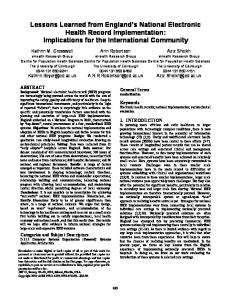
Fig. 1. Node placement at the greenhouses and the main paths to base station Pi07
Literature review reveals that in some cases network deployments were successful, but most of the presented examples can be just considered an important lesson. A deeper survey may be found in [6] where a number of real-life WSNs are analysed and conclusions are drawn. The article provides rules how to deploy networks to overcome reliability and prototype testing issues. The general conclusion is that even though propagation and energy consumptions models are usually known and carefully selected, the actual deployment still poses a lot of difficulties. These in turn affect the effectiveness of the selected solutions and there is a gap between what developers expect and what reality provides [8].
3
Testing setup
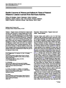
For our test deployment we used the well known and widely used TelosB nodes. They use protocol stack based on ZigBee and IEEE 802.15.4 standards and operate in 2.4 GHz wireless band (shared also by WiFi). We used four variants of the nodes, developed by Advanticsys (XM1000, CM3300, CM4000 and CM5000) that differ in antenna type (external 5 dBi or PCB), on-board sensor configuration and integrated programmer/USB interface. An example of two different node configurations can be seen in Fig. 2(a) and 2(b). Since all the nodes share the same programming environment, we find it beneficial to be able to compare e.g. communication ranges between different antennae types. Each wireless node is equipped with a set of sensors for measuring temperature, humidity and luminance in visible light spectrum (with 560 nm peak sensitivity wavelength), which are the base for environment monitoring in greenhouses [2]. The nodes operate on two AA rechargeable batteries with typical capacity of 2000 mAh.
A few selected nodes were also equipped with CO2 sensors, however their use was limited by the fact that the sensors required a separate 9 V energy source. Our test network was deployed in a relatively small greenhouse complex that is used for both teaching and research by the Wrocław University of Environmental and Life Sciences. It consists of a set of adjacent greenhouses, measuring 30×10 m each (Fig. 1). Each wireless node (T05, S42, etc.) was fixed to the support wires located approx. 3 m above the ground (see Fig. 2(a)). One base station (PI07) was placed in greenhouse B6, approx. 0.2 m above the ground. The other one (PI06) was located in the corridor, approximately 0.6 m above the ground. This resulted in better communication conditions between relatively distant nodes (as they maintained the Line of Sight (LoS)), than between the nodes and the BS. Each node was programmed with our custom GreenhouseMonitor application running under TinyOS. We used the standard Medium Access Control (MAC) implemented in TinyOS with the Low Power Listening (LPL) protocol as a way to conserve energy. Using LPL in our setup allowed to extend useful unattended operating time of the network from 4 to over 18 days. Methods of further network lifetime extension (e.g. using deep sleep modes, turning off LEDs or using more efficient routing) did not serve the goal of learning the network operation at the target site and will be used in future tests. To avoid making wrong assumptions about network operation we used flooding as message routing method. This also provided an opportunity to analyse which routing paths were used the most. Each node was programmed to take measurements from all of its sensors and generate a message every 30 s. This is much more frequent than necessary, considering the rate of change of conditions in the greenhouse, but allowed us to gather large amount of data for analysis.
4
Datasink architecture
The goal for the experiments described below was to create a setup for a datagathering system that could be deployed in the remote greenhouse and would allow unattended data acquisition from wireless sensor nodes for at least 2-3 weeks (or possibly much longer). For collecting the measurement data (i.e. the data sink) we have tested different setups, including laptop computers, however, for unattended operation, the best choice is a small embedded system (Fig. 3). In our research we have experimented with BeagleBoard and Raspberry Pi architectures. The BeagleBoard xM is a 3-year old embedded system platform running on OMAP ARM Cortex-A8 processor and costing around $125. The Revision-B board includes an ethernet port and 4 USB ports, allowing connection of external harddrives or WiFi dongles and it runs the OMAP version of the Linux operating system. Raspberry Pi is a fairly recent development board including the ARM11 processor, 512 MB of RAM, ethernet port and 2 USB ports, running Raspian Linux. It costs around $35. One of the most important problems with our system running on BeagleBoard was the filesystem instability. Although the general practice with all Unix
(a) WSN node
(b) BeagleBoard base station
Fig. 2. Elements of the WSN network installed in a greenhouse
S
ee W
om Nc
ion
icat
mun
ZigB ethernet or WiFi
sensors management / remote data retrieval
autonomous packet sink
Fig. 3. Architecture of the masurement system
systems is to never power down the system abruptly, without the proper shutdown, sometimes such power-downs are unavoidable. In our case we have twice lost a week worth of measurement when the whole filesystem was corrupted beyond repair. Hard resets or power-downs are hard to avoid in unattended system operation and may be caused by many reasons – power outages, greenhouse workers temporarily disconnecting the system, or finally – inability to properly shutdown the system with no network connection and no input devices. Inability to ensure data safety in such cases disqualified BeagleBoard systems for our use. With Raspberry Pi platform, our biggest problem was the USB support of the Raspian Linux distribution – the system was freezing as soon as the wireless node was accessed through the USB port. Research of various discussion fora revealed that it is a known problem, with the general consensus of blaming it on the outdated chip in the RS232-to-USB converter. Since the FT232BM chip is an integral part of the TelosB programmer, the only resolution to this problem was to change the booting parameters of the Raspian system to slow
down the transfer rate on the USB bus. The proper solution however would be to rewrite the kernel driver for the FT232 chip to behave properly and not to cause the system panic. The conclusion from this experience is that even though the Raspberry Pi platform is a fairly modern one and with a great potential for growth, there is a general lack of understanding in the open systems developers community, that not only the newest and shiniest gadgets should get their support, but also some older hardware which may still be in use. Another problem was the lack of permanent internet connection in the greenhouse installation. All modern distributions of Linux depend heavily on internet access for system updates and software installation, but it should be possible to run them as isolated systems once we have a desired system version. However, it took a lot of effort to configure the system for such a way of operation. The symptoms of malfunction included losing the networking card setup if the DHCP server was not available (thus, making the system inaccessible even over the peer-to-peer crossed-over cable connection with a laptop computer), inability to boot properly without the network access, or losing the local time during operation, even if it was properly set at the booting time. With the lack of a proper RTC hardware, this posed another category of problems as the data gathered has to be properly timestamped.
5
Observations
We have run several experiments from July 2012 until now (January 2013), but in this chapter we focus on results obtained from the data collected between 4th and 22nd of January 2013 in two different greenhouses (Fig. 1). During that time succulents and herbs (section 1 and 2) and tropical plants (section 3) grew in greenhouse B5. At the end of 2012, section 1 of the greenhouse B6 was filled with tomatoes seedlings while other sections were not used for cultivation. One aim of deploying wireless sensor network was to estimate its reliability, range and routing paths of radio communication. For that purpose, every node appended routing path information to the messages it sent. Table 1 presents ratios of messages that originated from each node and reached the base station with direct transmissions (when packets were received at the base station directly from the source node) and indirect transmissions (when packets were received only when retransmitted by other nodes). We also counted percentage of missing packets based on sequential numbers. Since broadcast communication was used, the same packet could reach the base station both directly and indirectly, therefore the sum of percentages may exceed 100% – this is especially true for nodes located close to the base station (i.e. T25, S42, T3). Routing path analysis clearly shows that no packet from nodes located in greenhouse B5 reached the base station PI06 directly. This is caused by the fact that heating and control equipment is located in-between both greenhouses and effectively blocks radio communication to the PI06 located 0.2 m above the ground. However, there are almost no obstacles between nodes located in greenhouses B5 and B6 as they are located 3 m above the ground. Consequently,
nodes T12 and T25 receive packets from nodes in B5 and retransmit them to the base station PI06. This explains the big number of indirect transmissions to PI06. Also, only 0.26% of packets from node T20 reached the PI06 (through either T12 or T25). Communication link reliability between T20 and T12, T25 is low due to distance and obstacles, so only a few hundreds of packets from node T20 were successfully received over the whole period of 18 days. Table 1. Percentage of messages that reached each of the base stations Source node
T03 T05 T09 T10 T20 P32 T12 T25 S42
BS 06 Percent of messages direct indirect missing 0.00 84.66 15.34 0.00 0.36 99.64 0.00 61.14 38.86 0.00 85.78 14.22 0.00 0.26 99.74 0.00 34.69 65.31 71.73 0.09 28.27 99.50 99.48 0.10 71.78 71.64 28.11
BS 07 Percent of messages direct indirect missing 29.01 69.12 24.24 62.30 0.30 37.69 14.18 54.84 39.67 11.63 54.12 43.12 0.00 0.50 99.50 0.08 21.20 78.80 65.15 7.92 34.62 89.22 89.39 7.92 54.93 62.51 35.19
Fig. 1 presents node placement and main routing paths from all the nodes to base station PI07 with thickness of arrows corresponding to the number of messages. Most of the messages received at PI07 were actually transmitted through node T12. This is a consequence of two facts: first, nodes in B6 greenhouse used transmission power that was 15dB higher than power used by nodes in B5 greenhouse; second, node T12 was the only node that had LoS visibility to the base station PI07. Higher transmission powers also enabled nodes T12, T25 and S42 to directly reach the base station more often then in case of nodes T03 and T05. For the same reason, significantly more packets from distant nodes (T09, T10, T20 and P32) were routed successfully through node T12 (routing through other nodes, e.g. P03 and P05 failed mostly due to lower transmission power). Figure 4 presents received signal strength indicator value (RSSI) of packets received at the base station PI07. RSSI parameter estimates radio signal power at receiver and depends mostly on transmission power, propagation conditions and distance. We expected that RSSI will change periodically with daily and weekly cycles due to people working in the greenhouses, but we could not find any correlation. Although RSSI values differ for each node (e.g. as a result of different transmission paths, distances and obstacles) radio propagation changes in similar way for all nodes. When using RSSI measurements to adjust transmission power, one needs to disregard small oscillations (of 1 or 2 dBm) that most likely result from inaccuracy of measurement and not the radio propagation itself. We have also used nodes to measure environmental conditions – temperature, relative humidity and light level. Figure 5 presents light level and temperature variations over three day period in two different greenhouses. It can be seen that temperature values exceeding 23◦ C on 5th and 7th of January correlate with high levels of light. In fact these two days were sunny and direct solar radiation
RSSI value at the base station no. 7 −78 −80
RSSI [dBm]
−82 −84 −86 −88 −90 −92
Node 5 Node 42 Node 25
−94 −96
13/01 05:11 13/01 17:36 14/01 06:01 14/01 18:26 15/01 06:52 15/01 19:17 16/01 07:42 16/01 20:07 17/01 08:32 Date and time
Fig. 4. Received signal strength indicator at base station PI07 from selected nodes
heated the sensors. On the contrary, there is no increase in temperature during January 6th and the light level is two orders of magnitude smaller as weather was cloudy on that day. Oscillations of temperature level (especially during the night) result from cyclic operation of central heating system. Small difference (1-1.5◦ C) between temperatures in both greenhouses results from different setup of heating system – increased temperature is provided to seedlings in B6 greenhouse. The light level plot also reveals increased light level between midnight and morning in greenhouse B6 (node S42). This is due to additional illumination provided during the night in this greenhouse for stimulated grow of plants. Another interesting observation was that constant environment monitoring can be used for alarming in critical situations. Fig. 6 shows a part of temperature profile collected during four days in November 2012. Normally the automated heating was supposed to keep the temperature around 23◦ C. However, a significant drop in temperature can be observed during the second night. It was caused by central heating unit malfunction and resolved in the morning. If it was not for the relatively mild thermal conditions outside, the crops might have been endangered.
6
Conclusions
When deploying a network that should run unattended for long time, reliability of the whole solution is the key factor. In most cases, remote access to network is difficult, relatively expensive and often non trivial. When available, remote access allows debugging the network and taking actions when unexpected situations take place. Therefore, on-site internet access greatly simplifies deployment, configuration and monitoring, and should be considered a necessity. Because contemporary simulation models are not accurate enough, network planning is an important part of the deployment process and all decisions (such as sensor locations) must be well thought. Our study shows that usually it is not possible to setup the network in laboratory and move it to the deployment area
Node 42 Node 10
Node 42 Node 10
26 25
3
24
Temperature [C]
Illumination [lx] (log scale)
10
2
10
23 22 21 20 19
1
10
18 17
05/01 10:56
05/01 23:21
06/01 11:46
07/01 00:11
07/01 12:36
05/01 10:56
05/01 23:21
06/01 11:46
07/01 00:11
07/01 12:36
Fig. 5. Light level (left) and temperature (right) measured in two different greenhouses over the same period of time. Note that light level is in log scale.
38 Node 10 Node 3
36 34
Temperature [C]
32 30 28 26 24 22 20
13/11 10:55
13/11 20:50
14/11 06:45
14/11 16:40
15/11 02:35
15/11 12:30
15/11 22:24
Fig. 6. Temperature in the greenhouse in a 4 days period
without any problems. This is so, since a number of parameters depend heavily on location, e.g. heights of antennas influence RSSI and effective communication range, propagation conditions depend on environment, obstacles and crop volume, spatial and temporal characteristics of the environment is different in laboratory and inside a greenhouse. We have observed some of these issues in our deployment even though it was thoroughly tested in laboratory: increased packet loss, difficulty in predicting routing paths, adverse interference from external environmental factors and also some seemingly trivial problems, such as the lack of power outlets to power the base stations. Our experiments show that there is an increasing need for improved tools for network planning. Such tools should not only use mathematical models of typical environments but also capture a variety of different aspects of radio transmission and wireless network deployment. Until then networks need to be planned for worst case scenario and thoroughly verified in the field before they are put in operation. This is crucial in precision agriculture applications but also in any application where failures may lead to tremendous and irreparable losses. During the deployment many typical engineering problems and challenges appeared (e.g. weak OS support for embedded hardware) which added extra workload to the team. Such problems are not possible to predict based only on
experiences with simulation-based research. It also follows from our study that WSN debugging and testing is difficult. Mainly due to the distributed nature of the system and constrained capabilities of a single node (limited memory, computational power, lack of remote access). Valuable simplification in this process was achieved by turning selected nodes into promiscuous mode. This allowed us to use dedicated software to sniff and debug all nearby communication. This gave us an insight into intra-node communication and operation. The experiences described here will allow for more complex deployment with dedicated and reliable routing. Our aim is to run the network for long period of time starting from early spring until the end of crop’s vegetation cycle.
Acknowledgment This work was supported by National Science Centre grant no. N 516 483740. The authors would like to thank Dr Piotr Chohura of Wrocław University of Environmental and Life Sciences for providing access to the greenhouses and valuable insights in the field of precision agriculture.
References 1. S. Blackmore, “Precision farming: an introduction,” Outlook on agriculture, vol. 23, no. 4, pp. 275–280, 1994. 2. K. Berezowski, “The landscape of wireless sensing in greenhouse monitoring and control,” International Journal of Wireless & Mobile Networks (IJWMN), vol. 4, no. 4, pp. 141–154, Aug. 2012. 3. K. Langendoen, A. Baggio, and O. Visser, “Murphy loves potatoes: experiences from a pilot sensor network deployment in precision agriculture,” in Parallel and Distributed Processing Symposium, 2006. IPDPS 2006. 20th International, Apr. 2006. 4. V. Jelicic, T. Razov, D. Oletic, M. Kuri, and V. Bilas, “MasliNET: A wireless sensor network based environmental monitoring system,” in MIPRO, 2011 Proceedings of the 34th International Convention, May 2011, pp. 150–155. 5. J. Xia, Z. Tang, X. Shi, L. Fan, and H. Li, “An environment monitoring system for precise agriculture based on wireless sensor networks,” in Mobile Ad-hoc and Sensor Networks (MSN), 2011 Seventh International Conference on, Dec. 2011, pp. 28–35. 6. T. Laukkarinen, J. Suhonen, T. Hamalainen, and M. Hannikainen, “Pilot studies of wireless sensor networks: Practical experiences,” in Design and Architectures for Signal and Image Processing (DASIP), 2011 Conference on, Nov. 2011, pp. 1–8. 7. W. Hu, T. L. Dinh, P. Corke, and S. Jha, “Outdoor sensornet design and deployment: Experiences from a sugar farm,” Pervasive Computing, IEEE, vol. 11, no. 2, pp. 82–91, Feb. 2012. 8. C. Di Martino, M. Cinque, and D. Cotroneo, “Automated generation of performance and dependability models for the assessment of wireless sensor networks,” Computers, IEEE Transactions on, vol. 61, no. 6, pp. 870–884, Jun. 2012.