Level Set based Reconstruction Algorithm for EIT Lung Images: First Clinical Results Peyman Rahmati1 , Manuchehr Soleimani2 , Sven Pulletz3 , In´ ez 3 1 Frerichs , and Andy Adler 1
Department of Systems and Computer Eng., Carleton University, ON., Canada Department of Electronic & Electrical Engineering, University of Bath, UK 3 Department of Anaesthesiology and Intensive Care Medicine, University Medical Centre Schleswig-Holstein, Campus Kiel, Kiel, Germany 2
E-mail:
[email protected],
[email protected],
[email protected],
[email protected],
[email protected] Abstract. We show the first clinical results using the level set based reconstruction algorithm for electrical impedance tomography data. The level set based reconstruction method allows reconstruction of non-smooth interfaces between image regions, which are typically smoothed by traditional voxel based reconstruction methods. We develop a time difference formulation of the level set based reconstruction method for 2D images. The proposed reconstruction method is applied to reconstruct clinical electrical impedance tomography data of a slow flow inflation pressure-volume manoeuvre in lung healthy and adult lung injury patients. Images from the level set based reconstruction method and the voxel based reconstruction method are compared. The results show comparable reconstructed images, but with an improved ability to reconstruct sharp conductivity changes in the distribution of lung ventilation using the level set based reconstruction method.
1. Introduction Tomographic imaging systems seek to see the inside objects, by introducing energy and measuring its interaction with the medium. Electrical Impedance Tomography (EIT) measures the internal impedance distribution using surface measurements. Electrical current is applied to the medium and the voltage at the surface is measured using electrodes. The impedance distribution is then estimated based on the measured voltages and medium geometry. Some of typical applications of these techniques are for geophysical imaging (Loke and Barker 1996a 1996b; Church 2006), process monitoring (Soleimani et al 2006a; Manwaring et al 2008), and functional imaging of the body (Frerichs 2000; Frerichs et al 2001; Gao et al 2006; Adler et al 2009; Frerichs et al 2010; Rahmati et al 2011; Pulletz et al 2011). In this paper, we focus on image reconstruction in EIT using the level set (LS) approach. The LS approach has become popular because of its ability to track
P. Rahmati et al
2
propagating interfaces (Osher and Sethian 1988; Sethian 1999), and more recently it has been applied in variety of applications in inverse problems and in image processing (Santosa et al 1996; Litman et al 1998; Dorn et al 2000; Osher and Paragios 2003). Level set based reconstruction method (LSRM) is a nonlinear inversion scheme using GaussNewton (GN) optimization approach to iteratively reduce a given cost functional, which is the norm of the difference between the simulated and measured data. In comparison to the voxel based reconstruction method (VBRM) ( e.g. Polydorides et al 2002), the LSRM has the advantage of introducing the conductivity of background and that of inclusions as known priori information into the reconstruction algorithm, enabling it to reconstruct sharp contrasts (Soleimani et al 2006a). The unknown parameters to be recovered from the data are the size, number, shapes of the inclusions. These unkown parameters are given as the zero LS of a higher dimensional function, called level set function (LSF). In every iteration, the LSF is modified according to an update formula to modify the shape of the inclusion at its zero LS (see figure 1). The LS method for shape based reconstruction is well studied in electrical and electromagnetic imaging for simulated and experimental tank data (Santosa et al 1996; Litman et al 1998; Dorn et al 2000, Boverman et al 2003; Chan and Thai 2004; Soleimani et al 2006b; Soleimani 2007; Banasiak and Soleimani 2010); however, it has been never shown to be used for clinical data. This study, along with our previous work (Rahmati et al 2011) are the first implementation of the LSRM using time difference data for EIT clinical data. In this study, we use a difference formulation of LSRM to reconstruct a 2D image of the distribution of lung ventilation over an inflation manouevre (figure 4 and figure 5). The remainder of the paper is organized as follows: in the next section, we formulate the image reconstruction algorithms using difference and absolute solvers for EIT (section 2.1). In subsection 2.2, we introduce into the LS technique employed for solving the inverse problem of EIT lung images. Subsection 2.3 discusses the details about the applied human data set, and the setting of the EIT system. In section 3, the experimental results are shown for the LSRM and the VBRM; and the performance of the difference mode LSRM for monitoring human lungs data is qualitatively and quantitatively compared with that of the VBRM. Section 4 presents discussions and conclusions. 2. Methods 2.1. Difference and absolute reconstruction methods There are two primary reconstruction types in EIT: “absolute (static) imaging” which attempts to recover an estimate of the absolute conductivity of the medium from the achieved data frame, and “difference imaging” which attempts to recover an estimate of the change in conductivity between two times based on the change between two data frames, v2 and v1 . Difference EIT can compensate for measurement errors which do
P. Rahmati et al
3
not change between data frames. Difference EIT is based on a difference data vector, [y]i = [v2 ]i − [v1 ]i , where i is the number of the measurements,or, to increase sensitivity to small measurements, the normalized difference data [y]i = ([v2 ]i − [v1 ]i )/[v1 ]i . Using a finite element model (FEM), the medium is discretized into N elements with conductivity σ. The conductivity change vector x = σ2 − σ1 is the change between the present conductivity distribution, σ2 , and that at the reference measurement, σ1 . The linearized difference forward solution for small changes in conductivities over time is given by (Adleret al 2007): y = Jx + n,
(1)
where J is Jacobian or sensitivity matrix around the reference conductivity ∂y |σ1 and n is the measurement noise, typically assumed to distribution, defined by ∂x be an uncorrelated white Gaussian noise. In EIT, we need to solve an inverse problem to find an estimate of the conductivity, refered to as xˆ. The most common approach to find xˆ is the use of the Gauss-Newton (GN) algorithm for EIT reconstruction (Cheney et al (1990)). The GN method solves the EIT inverse problem by minimizing the the following quadratic residue (Adleret al 2007): ky − J xˆk2P−1 + kˆ x − x0 k2P−1 , n
(2)
x
where −1 and xˆ−1 are the covarience matrix of measurement noise and that of n conductivity vector (ˆ x), respectively; and x0 represent the expected value of element conductivity changes. By solving (2) for xˆ, the linearized EIT inverse solution is obtained as (see Appendix A): P
P
xˆ = (J T J + R)−1 (J T y + Rx0 ),
(3)
where R is the regularization matrix and x0 is the initial guess of the solution, which can be assigned to zero. In the remainder of this paper, the GN approach is considered the reference technique. GN image reconstruction typically results in smoothed images with blur edges, since the regularization matrix is based on a penalty filter for non-smooth images. 2.2. Level set method One effective method to allow the reconstruction of sharp images is the LS method (Dorn et al 2000). The classic formulation of this method assumes that the reconstructed image can take only two conductivity values: one for background with value σb and another one for inclusions with value σi . The regions which form the background and the inclusions are defined by the LSF, Ψ: a signed distance function to identify the unknown interface between the two conductivities. The value of the LSF is zero on the interface, negative inside the interface, and positive outside. Compared to the more typical VBRMs, the LSRMs allow more accurate reconstruction of the boundary shape of step changes of conductivity (high contrast objects). This is because most regularization schemes for the traditional methods, which
P. Rahmati et al
4
are necessary for stabilizing the inversion, have the side-effect of artificially smoothing the reconstructed images. Therefore, these schemes are not well-suited for reconstructing high contrast objects with sharp boundaries. In order to arrive at a robust and efficient shape-based inversion method, there is a requirement to computationally model the moving shapes. The LS technique (Osher and Sethian, 1988; Sethian, 1999) is capable of modeling the topological changes of the boundaries. Figure 1 shows a two phases image reconstructed using the LSRM. The LSF Ψ has separated the zero LS surface into two regions: foreground (inclusions) and background. The mapping function Φ projects the LSF to a 2D mesh to be applied for inverse solution calculation using FEM. Figure 1, right panel, shows the conductivity of the inclusions in black where the LSF is negative and that of background in white where the LSF is positive. To begin with, we need to define an initial LSF, which may be a circle on level zero; and then deform this inital LSF using a predefined energy functional iteratively. Figure 2 represents the steps as k represents the iteration number. After defining the initial LSF, the mapping function Φ projects the LSF to a 2D mesh to be fed to difference solver block to calculate the system senitivity matrix, Jacobian (Jk ), as well as differential potential vectors, ∆di = [dreal ]i − [d(simulated)]i . The next step is to update the energy functional via a Gauss-Newton formula, ∆LSFk . The initial LSF is then deformed by ∆LSFk generating a new LSF. This new LSF is fed again to difference solver block for another iteration if the current iteration number (k) is not bigger than a maximum iteration number (K). In the following, we discuss about the mathematical presentation of the LSRM. In this technique, the shapes which define the boundaries, are represented by the zero LS of a LSF Ψ. If D is the inclusion with conductivity σi embedded in a background with conductivity σb , the boundary of the inclusion, which is also an interface between two materials, is given by the zero LS (Soleimani et al 2006b): ∂D := {r : Ψ(r) = 0},
(4)
where the image parameter at each point r is (Soleimani et al 2006b) σi
for {r : Ψ(r) < 0}
σb
for {r : Ψ(r) > 0}
σ(r) =
,
(5)
If we change this LSF for example by adding an update, we move the shapes accordingly. This update to a given LSF causes the shapes being deformed in a way which reduces an error residue (cost functional). The LSRM combines the general idea of GN optimization approach with a shapebased inversion approach. To derive the LSRM, we define the mapping (Φ) which assigns a given LSF ΨD to the corresponding parameter distribution by σ = Φ(ΨD ). The parameter distribution σ has the same meaning as in the traditional GN inversion scheme. The only difference is that in the shape-based situation it is considered as having only two values, namely an “inside” value and an “outside” value. In shapebased reconstruction approach, we are looking for the LSF ΨD which divides the image into two separate areas as foreground (inclusion) and background.
P. Rahmati et al
5
Having defined this mapping Φ, we can now replace the iterated parameter σk , with the definition defined in (5), by σk = Φ(ΨD ) = Φ(Ψk ). Instead of the forward mapping F (σ), where function F maps the electrical conductivity distribution to the measured data, we need to consider now in the new GN type approach the combined mapping (Soleimani et al 2006b): d(Ψ) = G(Φ(Ψ)),
(6)
where d is data point matrix, G is system matrix, and Φ(Ψ) stands for conductivity, see figure 1.
Ψ (Level set function)
Φ (Mapping function) Zero level set function(LSF=0)
σ (conductivity)=Φ(Ψ)
Figure 1: Level set function mapping to a 2D plane. From left to right columns, The 3D representation of an arbitarary level set function and its zero level set function crossing zero level set surface, and 2D mapping of the leve set function on the zero lever set surface. According to the chain rule, the LS sensitivity matrix (JLS ) can be written as below: JLS =
where
∂G ∂Φ(Ψ)
∂G ∂Φ(Ψ) ∂d =( )( ) ∂Ψ ∂Φ(Ψ) ∂Ψ = (JGN )(M ),
(7)
stands for the traditional GN sensitivity matrix (JGN ), and we define
∂Φ(Ψ) ∂Ψ
= M . Then, the new GN update (Soleimani et al 2006b) is as follows (see Appendix A) : h
i
T T Ψk+1 = Ψk + λ (J(LS,k) J(LS,k) + α2 LT L)−1 (J(LS,k) (dreal − d(Ψk )))
h
i
− α2 LT L(Ψk − Ψint ) = Ψk + GNupdate = LSF (k) + ∆LSF,
(8)
where Ψint in the update term corresponds to the initial esimate of the LSF. There are two parameters λ and α to be tuned in this LS formulation. Figure 2 illustrates the algorithm to calculate the above update formula. The optimal choice of the two parameters, λ and α, depends on the mesh density, the conductivity contrast and the initial guess (Soleimani et al 2006a). The length parameter λ and the α both
P. Rahmati et al
6
affect the magnitude of the LSF displacement; however, λ makes the main effect on the displacement, changing the shape of inclusion, in a given update. The higher the λ, the higher the LSF displacement will be. The effect of the regularization parameter α depends on the choice of the regularization operator L. An identity matrix for L increases the stability of the inversion by reduced smoothing of the LSF. However, a first order difference operator for L will smooth the LSF (Soleimani et al 2006a). As α increases, the smoother the final LSF tends to be. A large value for α prevents the reconstruction algorithm from being able to separate close objects (low distinguishibility). In our experiments, the choice of L as the identitiy operator was made to improve distinguishibility. In our results, we have put a value of zero for our initial guess of Ψint in the above shape-reconstruction form. 2.3. Experimental data Experimental data were obtained in the study described by Pulletz et al (2011). Briefly, human breathing data were acquired from eight patients with healthy lungs (age: 41 ± 12 years, height: 177 ± 8 cm, weight: 76 ± 8 kg, mean ± std.) and eighteen patients (age: 58 ± 14 years, height 177 ± 9 cm, weight: 80 ± 11 kg) with acute lung injury (ALI). All patients were intubated and mechanically ventilated. The experimental proceedure consisted of a low flow inflation pressure-volume manoeuvre applied by the respirator (Evita XL, Draeger, Luebeck, Germany), starting at an expiratory pressure of 0 cmH2O and ending when either a) the gas volume reached 2L, or b) the measured airway pressure reached 35 cmH2O. Airway gas flow, pressure and volume were recorded at a sampling rate of 126 Hz. An example pressure curve during the inflation protocol is shown in Figure 4. EIT data were acquired on sixteen self-adhesive electrodes (Blue Sensor L-00-S, Ambu, Ballerup, Denmark), placed at the 5th intercostal space in one transverse plane around the thorax, while a reference electrode was placed on the abdomen. EIT data were acquired at 25 frames per second, with an adjacent stimulation and measurement protocol, using current stimulation at 50 kHz and 5 mArms. Overall, 477 EIT data frames are acquired per inflation manoeuvre. 3. Experimental results Images were reconstructed on a mesh roughly conforming to the anatomy of the subject, and the two different reconstruction algorithms (the VBRM and the LSRM) were tested on the clinical data (figure 3 - figure 6). Figure 3 shows the reconstructed images of ventilation in a lung healthy patient measured based on the difference signal between start and end inflation. As inspired air increases, the resistivity of the lungs increases which has been shown as blue regions in the reconstructed images in figure 3. The reconstructed images clarify the difference between LSRM and VBRM in terms of creating sharper reconstructions with larger contrasts at the interface between
P. Rahmati et al
7 START
Initial guess of LSF (k=0)
3D representation of level set function
Δd= dm-dk
Real data
Reconstructed image at k
Simulated data
k=k+1
YES
Jacobian(Jk) update
Gauss-Newton (GN) update ΔLSF(update)
NO
END
K