Limitations of quantum computing with Gaussian cluster states

Limitations of quantum computing with Gaussian cluster states M. Ohliger1 , K. Kieling1 , and J. Eisert1,2

arXiv:1004.0081v2 [quant-ph] 17 May 2010

1

Institute of Physics and Astronomy, University of Potsdam, 14476 Potsdam, Germany and 2 Institute for Advanced Study Berlin, 14193 Berlin, Germany (Dated: May 18, 2010)

We discuss the potential and limitations of Gaussian cluster states for measurement-based quantum computing. Using a framework of Gaussian projected entangled pair states (GPEPS), we show that no matter what Gaussian local measurements are performed on systems distributed on a general graph, transport and processing of quantum information is not possible beyond a certain influence region, except for exponentially suppressed corrections. We also demonstrate that even under arbitrary non-Gaussian local measurements, slabs of Gaussian cluster states of a finite width cannot carry logical quantum information, even if sophisticated encodings of qubits in continuous-variable (CV) systems are allowed for. This is proven by suitably contracting tensor networks representing infinite-dimensional quantum systems. The result can be seen as sharpening the requirements for quantum error correction and fault tolerance for Gaussian cluster states, and points towards the necessity of non-Gaussian resource states for measurement-based quantum computing. The results can equally be viewed as referring to Gaussian quantum repeater networks.

I.

INTRODUCTION

Optical systems offer a highly promising route to quantum information processing and quantum computing. The seminal work of Ref. [1] showed that even with linear optical gate arrays alone and appropriate photon counting measurements, efficient linear optical computing is possible. The resource overhead of this proof-of-principle architecture for quantum computing was reduced, indeed by orders of magnitude, by directly making use of the idea of measurement-based quantum computing with cluster states [2–4]. Such an approach is appealing for many reasons, the reduction of resource overheads only being one, but also for a clearcut distinction between creation of entanglement as a resource and its consumption in computation. This idea was further developed into the continuous-variable (CV) version thereof [5–8], aiming at avoiding limitations related to efficiencies of creation and detection of single photons. In this context, Gaussian states play a quite distinguished role as they can be created by passive optics, optical squeezers and coherent states, i.e., the states produced by a usual laser [9–13]: Indeed, Gaussian cluster states form a promising resource for instances of quantum computing with light. Such a CV-scheme allows for a deterministic preparation of the resource states while the schemes based on linear optics with single photons require preparation methods which are intrinsically probabilistic. In this work, we however highlight and flesh out some limitations of such an approach. We do so in order to sharpen the exact requirements that any scheme for CV quantum computing based on Gaussian cluster states eventually will have to fulfill, and what quantum error correction and fault tolerant approaches eventually have to deliver. Specifically, we will show that Gaussian local measurements alone will not suffice to transport quantum information across the lattice, even on complicated lattices described by an arbitrary graph of finite dimension: Any influence of local measurements is confined to a local region, except from exponentially suppressed corrections. This can be viewed as an impossibility of Gaussian error correction in the measurement-based setting. What is more, even under non-Gaussian measurements, this obstacle

(a)

(b)

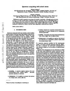
FIG. 1. GPEPS on an arbitrary graph, here one representing a cubic lattice. (a) The connected dots represent two-mode squeezed states, the circles denote the vertices where the Gaussian projections are being performed. (b) The resulting GPEPS after local Gaussian projections have been performed on the virtual systems. Any Gaussian cluster state can be prepared in this fashion.

cannot be overcome, in order to transport or process quantum information along slabs of a finite width: Any influence of local measurements will again exponentially decay with the distance. This observation suggests that—although the initial state is perfectly known and pure—finite squeezing has to be tackled with a full machinery of quantum error correction and fault tolerance [14–16], yet to be developed for this type of system and presumably giving rise to a massive overhead. No local measurements or suitable sophisticated encodings of qubits in finite slabs—reminding, e.g., of encodings of the type of Ref. [16]— can uplift the initial state to an almost perfect universal resource. In order to arrive at this conclusion, in some ways, we will explore ideas of measurementbased computing beyond the one-way model [2] as introduced in Ref. [17] and further developed in Refs. [18–22]. We will highlight the technical results as “observations”, and discuss implications of these results in the main text. While these findings do not constitute a “no-go” argument for Gaussian cluster states, they do seem to require a very challenging prescription for quantum error correction and further highlight the need for identifying alternative schemes for CV quantum computing, specifically ones based on non-Gaussian CV

2 states. Small scale implementations of Gaussian cluster state computing are, as we will see, are also not affected by these limitations. To sketch the structure of this article: In Section III we will first discuss the concept of Gaussian projected entangled pair states (GPEPS), forming a family of states including the physical CV Gaussian cluster state. In Section IV we will then discuss the impact of Gaussian measurements on GPEPS and show that under this restriction the localizable entanglement in every GPEPS decays exponentially with the distance between any two points on arbitrary lattice. This has also implications on Gaussian quantum-repeaters, which we investigate in detail. After this, we leave the strictly Gaussian stage in Section V and investigate present our main result when showing that under more general measurements on GPEPS, quantum information processing in finite slabs is still not possible. We discuss requirements for error correction, before presenting concluding remarks.

II.

PRELIMINARIES

A.

Gaussian states

Before we turn to measurement-based quantum computing (MBQC) on CV-states, we briefly review some basic elements of the theory of Gaussian states and operations which are needed in this article [9–12]. Readers familiar with these concepts can safely skip this section. Although the statements made in this work apply on all physical systems described by quadratures or canonical coordinates, including, e.g., micromechanical oscillators, we have a quantum optical system in mind and often use language from this field as well. Any system of N bosonic degrees of freedom, e.g., N light modes, can be described by canonical coordinates xn = (an + a†n )/21/2 and pn = −i(an − a†n )/21/2 , n = 1, . . . , N , where an (a†n ) annihilates (creates) a photon in the respective mode. When we collect these 2N canonical coordinates in a vector O = (x1 , p1 , . . . , xN , pN ), we can write the commutation relations as [Oj , Ok ] = iσj,k , where the symplectic matrix σ is given by σ=

 N  M 0 1 . −1 0

(1)

j=1

Gaussian states are fully characterized by their first and second moments alone. The first moments form a vector d with entries dj = tr(Oj ρ) while the second moments, which capture the fluctuations, can be collected in a 2N × 2N -matrix γ, the so-called covariance matrix, with entries γj,k = 2Re tr [ρ (Oj − dj ) (Ok − dk )] .

(2)

Hence, Gaussian states are complete characterized by d and γ. Gaussian unitaries, i.e., unitary transformations acting in Hilbert space preserving the Gaussian character of the state correspond to symplectic transformations on the CM. They in turn correspond so maps γ 7→ SγS T with SσS T = σ.

The set of such symplectic transformations forms the group Sp(2N, R). A set of particularly important example Gaussian states are the coherent states, for which the state vectors read in the photon number basis 2

|αi = e−|α|

/2

∞ X αn √ |ni n! n=0

(3)

and are described by d = (Re α, Im α) and γ = diag(1, 1). Single mode squeezed states are characterized by lower fluctuations in one phase-space coordinate. The CM can in a suitable basis then be written as γ = diag(x, 1/x) with x 6= 0. B.

MBQC on Gaussian cluster states

The first proposal for MBQC on CV states has been based on so-called Gaussian cluster states and works in almost complete analogy to the qubit case [5–8]. As such, the formulation is based on “infinitely squeezed” and hence unphysical states using infinite energy in preparation: It can be created by initializing every mode in the p = 0 “eigenstate” of p (formally an improper eigenstate of momentum, a concept that can be made rigorous, e.g., in an algebraic formulation [25]). This is the CV-analogue to the state vector |+i = (|0i + |1i)/21/2 in the qubit case. Then the operation eix⊗x , the analogue to the CZ gate, is applied between all adjacent modes. This state allows universal MBQC to be performed with Gaussian and one non-Gaussian measurement. The state as such is not physical and not contained in Hilbert space. The argument, however, is that it should be expected that a finitely squeezed version inherits essentially the same properties. Replacing them by finitely squeezed ones we obtain a state which we will call a physical Gaussian cluster state. III.

GAUSSIAN PEPS

Projected entangled pair states (PEPS) or tensor product states have been used for qubits to generalize matrix product states (MPS) or finitely correlated states [26, 27] from onedimensional chains to arbitrary graphs [28–30]. One suitable of defining them is via a valence-bond construction: One can create a state by placing entangled pairs—constituting “virtual systems”—on every bond of the lattice and then applying a suitable projection to a single mode at every lattice site. These projections, often taken to be equal, together with the specification of the initial entangled states, then serve as a description of the resulting state. MPS for Gaussian states (GMPS) have been studied to obtain correlation functions and entanglement scaling in one-dimensional chains [31]. In this work we focus on Gaussian PEPS (GPEPS) which can be obtained from non-perfectly entangled pairs. The bonds we consider are two-mode squeezed states (TMSS), the state vectors of which have the photon number representation |ψλ i = (1 − λ2 )1/2

∞ X n=0

λn |n, ni,

(4)

3 where λ ∈ (0, 1) is the squeezing parameter. We will denote the corresponding density matrix by ρλ . For λ → 1 the state becomes “maximally entangled”, but this limit is not physical because it is not normalizable and has infinite energy as already mentioned above. We will, therefore, carefully analyze the effects stemming from the fact that λ < 1. The covariance matrix of this state reads   cosh(2r) 0 sinh(2r) 0 0 cosh(2r) 0 −sinh(2r)   γλ =   (5) sinh(2r) 0 cosh(2r) 0 0 −sinh(2r) 0 cosh(2r) where tanh(r/2) = λ. This number r will also be referred to as the squeezing parameter in case there is no risk of mistaking one for the other. It is also known that any pure bipartite multi-mode Gaussian state can be brought into the tensor product of TMSS [10, 32] by means of local unitary Gaussian operations, each having a CM in the above form. Then the largest r in the vector of resulting TMSS will be referred to as its squeezing parameter. We will also discuss GPEPS on general graphs G = (V, E), as shown in Fig. 1. Vertices G here correspond to physical systems, edges E to connections of neighborhood. On any such graph, d(., .) is the natural graph-theoretical distance between two vertices. As we will often consider the system of bonds before the projection operation is performed, we employ the following notation: When we speak of operations on virtual systems when thinking of collective operations on modes before the projection is applied, and often emphasize when we refer to a single physical system with Hilbert space H = L2 (R). Note that we also allow for more than one edge between two vertices of a graph. When a particular vertex has N adjacent bonds, the projection map is a Gaussian operation of the form V : H⊗N → H.

(6)

This operation can always be made trace-preserving [9, 12, 23, 24], in quite sharp contrast to the situation in the finitedimensional setting. This operation will also be referred to as Gaussian PEPS projection. This operation can always be realized by mixing single-mode squeezed state on a suitably tuned beam splitter which means that inline squeezers are not necessary [33]. Note that any such state could also be used as a variational state to describe ground states of many-body systems and by construction satisfies an entanglement area law [34]. IV.

GAUSSIAN OPERATIONS ON GPEPS

In this section, we will discuss Gaussian operations on a GPEPS and derive some statements on entanglement swapping, the localizable entanglement, and the usefulness as a resource for MBQC. Since all measurements are assumed to be Gaussian as well, this is as such not yet a full statement on universality, but already shows that the natural operations for transport of logical information in such a Gaussian cluster state does not work with such local measurements.

A.

Localizable entanglement

The localizable entanglement (LE) between two sites A and B of the graph G = (V, E) is defined by the maximal entanglement obtainable on average when performing projective measurements at all sites but A and B [35]. When we require both the initial state and the measurements to be Gaussian [36, 37], the situation simplifies as the entanglement properties do not depend on the measurement outcomes [9, 12, 23, 24]. Thus, we do not need to average but only find the best measurement strategy. To be specific, we will measure the entanglement in terms of the logarithmic negativity which can be defined as [38–40] E(ρ) = logkρTA k1 ,

(7)

where TA denotes the partial transpose with respect to subsystem A and k.k1 the trace-norm and we use the natural logarithm. For a TMSS, E coincides with the squeezing parameter by E(ρλ ) = r. It is important to note, however, that this choice has only been made for notational convenience: In our statements on asymptotic degradation of entanglement, any other measure of entanglement would also do, specifically the entropy of entanglement for pure Gaussian states, and for mixed states the distillable entanglement or the entanglement cost. We will mostly focus on two variants of the concept of localizable entanglement: Whenever we only allow for Gaussian local measurements, we will refer to this quantity as Gaussian localizable entanglement, abbreviated as EG . Then, we will consider the situation when we ask for fixed subspaces SA and SB in the Hilbert spaces associated with sites A and B to get entangled by means of local measurements. We then refer to as subspace localizable entanglement ES . Both concept directly relate to transport in measurement-based quantum computing. B.

Entanglement swapping

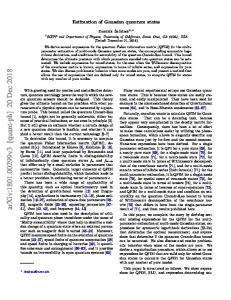
The task of localizing entanglement in a PEPS is closely related to one of entanglement swapping [41]. In this situation we have three parties, A, B, and C where both A and B and B and C share an entangled pair each. Then B, consisting of B1 and B2 , is allowed to perform an arbitrary Gaussian operation on his parts of the two pairs followed by a measurement. The task is to choose the operation in such a way that the resulting entanglement between A and B is maximum. Lemma 1 (Optimality of Gaussian Bell measurement for entanglement swapping of two-mode squeezed states). For two pairs of entangled TMSS shared between A and B1 and B1 and C, the supremum of maximum achievable negativity between A and C by a local Gaussian measurement in B1 , B2 is approximated by the measurement that best approximates a Gaussian Bell measurement. We consider the situation of having a TMSS (5) |ψiA,B1 = |ψλ1 iA,B1 , |ψiB2 ,C = |ψλ2 iB2 ,C

(8)

4 holds, since Y Z −1 Y T ≥ 0. Therefore, 0 γA,C = γA,C +P

FIG. 2. Situation referred to in Lemma 2. The strongest bonds before the projection are r1 and r2 . The most significantly entangled bond has the strength f (r1 , r2 ).

with some λ1 , λ2 > 0 and restricting the operation on B to be Gaussian. Furthermore, we allow for operations which do not succeed with unit probability. We have to allow for general local Gaussian operations, and also for arbitrary local additional Gaussian resources, with CM γB on modes B3 , on an arbitrary number of modes. The initial covariance matrix of the system hence reads γ = γλ1 ⊕ γλ2 ⊕ γB3 .

(9)

Without loss of generality, one can assume that one performs a single projection onto a pure Gaussian state on all modes referring to B. Ordering modes to A, C, B1 , B2 , B3 , one can write the CM in block form as   U V 0 γ =  V T W 0 , (10) 0 0 γB3 U referring to A, C and V to B1 , B2 . When we now project the modes B1 , B2 , and B3 onto a pure Gaussian state with CM Γ, the CM of the resulting state of A and C, postselected on that outcome, is given by the Schur-complement [9, 23, 24],   −1  T      U 0 W 0 V − V 0 +Γ . γA,C = 0 0 0 γB3 0 (11) Any symplectic operation S applied to B before the measurement can of course also be just absorbed into the choice of the CM Γ. Writing     X Y W 0 +Γ= , (12) 0 γ B3 YT Z one finds that the left upper principal submatrix of the inverse can be written as  −1 X Y = (X − Y Z −1 Y T )−1 , (13) YT Z B1 ,B2

again in terms of a Schur complement expression. Since γB3 + iσ ≥ 0 and the same holds for the subblock on B3 of Γ, these matrices are clearly positive. Using operator monotonicity of the inverse function, one finds that (X − Y Z −1 Y T )−1 ≥ 0

(14)

(15)

0 with a matrix P ≥ 0. Here γA,C is the CM following the same protocol, but where Γ is replaced by the identical CM, but with Y = 0. To arrive at such a CM is always possible and still gives rise to a valid CM by virtue of the pinching inequality. This is yet merely the covariance matrix of the a Gaussian state, subjected to additional classically correlated Gaussian noise. In other words, it is always optimal to treat B3 as an innocent bystander and not to perform an entangling measurement between B1 and B2 on the one hand and B3 on the other hand, quite consistent with what one could have intuitively assumed. We can hence focus on the situation when B3 is absent and we merely project onto a pure Gaussian state in B1 and B2 . It is then easy to see that there is no optimal choice, but the supremum can be better and better approximated by considering more and more squeezed TMSS (or “infinitely squeezed states” in the first place), i.e., on |ψλ i in the limit of λ → 1, which is the CV-analogue to the Bell state for qudits. This measurement can be realized by mixing B1 and B2 on a beam splitter with reflectivity R = 1/2 and performing homodyne measurement on both modes afterwards (i.e., a projection on a infinitely squeezed single-mode state being improper eigenstates of the position operator). From Eqs. (5) and (11) with Γ = γλ and performing the limit λ → 1, we can calculate the CM of the resulting state. It has the form of (5) with

r = f (r1 , r2 ) =

1 1 + cosh2r1 cosh2r2 arcosh . 2 cosh2r1 + cosh2r2

(16)

We note that f is symmetric in its arguments and fulfills f (r1 , r2 ) < min{r1 , r2 } and limr1 →∞ f (r1 , r2 ) = r2 . This means, arbitrarily faithful entanglement swapping is possible exactly in the limit of infinite entanglement. Otherwise the entanglement necessarily deteriorates [41]. To show that this measurement is indeed optimal, we set Γ = Sγλ S T

(17)

where S ∈ Sp(4, R). Calculating the resulting degree of entanglement, a direct and straightforward inspection reveals that E(ρA,C ) can only decrease whenever we choose S 6= 1. C.

One-dimensional chain

We now turn to a one-dimensional GPEPS, not allowing multiple bonds in the valence-bond construction, and are in the position to show the following observation: Observation 1 (Exponential decay of Gaussian localizable entanglement in a 1D chain). Let G be a one-dimensional GPEPS and A and B two sites. Then EG (A, B) ≤ c1 e−d(A,B)/ξ1

(18)

where c1 , ξ1 > 0 are constants. The best performance is reachable by passive optics and homodyning only.

5 In order to prove this, we interpret the preparation projection (6) and the following measurements of the localizable entanglement protocol as a sequence of instances of entanglement swapping. Clearly, to allow for general Gaussian projections is more general than (i) using the specific Gaussian projection of the PEPS, followed by a (ii) suitable Gaussian projection onto a single mode; hence every bound shown for this setting will also give rise to a bound to the actual 1D Gaussian chain. If d(A, B) is again the graph-theoretical distance between A and B we have to swap k = d(A, B) − 1 times. Defining g(r) = f (r, rI ) where rI is the initial strength of all bonds and iterating the argument we obtain rA,B = (g ◦k )(rI ) = F (k) .

(19)

As the negativity is up to a simple rescaling equal to this two-mode-squeezing parameter, the only task left is to show that F (k) decays exponentially. In order to do this, we need arcosh(x) = log(x + (x2 − 1)1/2 ) and the following relations which hold for x ≥ 0: cosh(x) ≥ ex /2, cosh(x) ≤ ex . With the help of them, we can conclude that F (k + 1)/F (k) < Q < 1

(20)

for a Q only depending on rI . Thus, F (k) decays exponentially which proves Observation 1. Note that in order to maximize the entanglement between A and B, we have chosen the supremum of the maps better and better approximating the projection onto an infinitely entangled TMSS. Thus, for a specific GPEPS which is characterized by a fixed map V , the EG in generally lower. This result has a remarkable consequence for Gaussian quantum repeaters lines: It is not possible to build a onedimensional quantum repeater relying on Gaussian states, if only local measurements and no distillation steps are being used. We will show in Section V that even non-Gaussian measurements cannot improve the performance. If one sticks to the Gaussian setting, also relying on complex networks does not remedy the exponential decay, as we will see. Of course, non-Gaussian distillation schemes can be used in order to realize CV quantum repeater networks. D.

General graphs in arbitrary dimension

One should suspect that the exponential decay of EG is a special feature of the one-dimensional situation and that higher dimensional graphs would eventually allow to localize a constant amount of entanglement. In this section we will show that this is not the case. We first need a Lemma which follows directly from our discussion of entanglement swapping. Lemma 2 (Collective operations on pure Gaussian states). Let ρA,B1 be a pure Gaussian state on H⊗2n of n modes and ρB2 ,C a pure Gaussian H⊗2m state, where one part of each is held by A, B, and C, respectively. Let the maximum two-mode squeezing parameter be r1 between A and B and r2 between B and C. Then the maximum two-mode-squeezing parameter achievable with a Gaussian projection in B between A and C is f (r1 , r2 ).

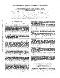
FIG. 3. Partitioning of the graph according to the shortest path as described in the main text. The sites drawn as squares are the ones which lie on the shortest path connecting A and B.

To prove this, we again use the fact that any two-party multi-mode pure Gaussian state can be transformed by local unitary Gaussian operations on both parties into a product of TMSS [10, 32]. This is nothing but the Gaussian version of the Schmidt decomposition. It does hence not restrict generality to start from that situation. As noted above, the best strategy for entanglement-swapping between two pairs is a Gaussian Bell-measurement, where the squeezing parameter changes according to f . We will now allow for global Gaussian operations on all subsystems belonging to B. This situation we will relax to the following, where we allow for even more general operations: Namely a local Gaussian operation onto all modes of B, as well as onto all modes of A and C that are not the two modes that share the largest r. Clearly, this is a more general map than is actually considered in the physical situation. This, however, is exactly the situation considered above, of an entanglement swapping scheme with an unentangled bystander. Hence, we again find that to project each pair onto a two-mode pure Gaussian state is optimal. For that, the sequence of projections better and better approximating infinitely squeezed TMSS gives rise to the supremum. Hence, we have shown the above result. Now we can prove a central result of this work. Observation 2 (Exponential decay of Gaussian localizable entanglement of GPEPS on general graphs). Consider a GPEPS on a general graph with finite dimension and let A and B be two vertices of this graph. Then there exist constants c2 , ξ2 > 0 such that EG (A, B) ≤ c2 e−d(A,B)/ξ2 .

(21)

We take the shortest path between A and B—achieving the graph-theforetical distance d(A, B)—and denote its vertices by A, v1 , . . . , vd(A,B)−1 , B. We partition the graph in such a way that the boundaries do not intersect or touch each other and every vertex on the shortest path from A and B is contained in one region which is called Rv (see Fig 3). Again we consider the situation of having TMSS distributed on the graph between vertices sharing an edge: A general local Gaussian measurement on a Gaussian PEPS—so the Gaussian PEPS projection now on several modes, followed by a specific single-mode Gaussian measurement can only be less general than a general collective Gaussian measurement, so again we will arrive at a bound to the localizable entanglement in the Gaussian PEPS.

6 E.

Remarks on Gaussian repeater networks

These results of course also applies to general quantum repeater networks, where the aim is to end up with a highly entangled pair between any two points in the repeater network (see, e.g., Ref. [44] for a qubit version thereof). That is, in Gaussian repeater networks, one will also need non-Gaussian operations to make the network work, quite consistent with the findings of Refs. [9, 23, 24].

FIG. 4. Exponential decay of any influence of any measurements of measurements in region I to statistics of measurement outcomes in O in the graph theoretical distance d(I, O) between the regions.

Now, we face exactly the situation to which Lemma 2 applies. In fact, we will in each step in each of the parts A, B, and C have a collection of TMSS, shared across the cut of the three regions. If rAv1 is the strongest bond, in terms of the two-mode squeezing parameter, between RA and Rv1 and rv1 v2 the strongest one between Rv1 and Rv2 , then the strongest bond between RA and Rv2 is given according to Lemma 2 by f (rAv1 , rAv2 ). Now, we can proceed exactly as in the proof of Theorem 1—and again any uncorrelated bystanders will not help to improve the degree of entanglement—and thus show Theorem 2. This has again a consequence for quantum repeaters: Even when an arbitrary number of parties can share arbitrary many Gaussian entangled bonds, it is not possible to teleport quantum information over an arbitrary distance as shown below. In fact, using this statement, one can show that any impact of measurements in terms of a measurable signal in confined to a finite region on the graph, now a I being a subset of the graph, expect from exponentially suppressed corrections. This region could be a poly-sized region in which the input to the computation is encoded. The read-out of the quantum computation is then estimated from measurements on some region O, giving rise to a bit that is the result of the original decision problem that is to be solved by the quantum computation. From the decay of localizable entanglement, it is not difficult to show that the probability distribution of this bit is unchanged by measurements in I, except from corrections that are exponentially decaying with d(I, O), see Fig. 4. Note that concerning small scale, “proof-of-principle” applications, the presented arguments do not impose a fundamental restriction as they only apply to the situation where entanglement distribution over an arbitrary number of modes (or repeater stations) is required. For any finite distance d(A, B) and required entanglement E(A, B) there exists a finite minimal squeezing λmin which allows to perform the task. Only asymptotically, one will necessarily encounter this situation. The result can equally be viewed as an impossibility of Gaussian quantum error correction in a measurement-based setting, complementing the results of Ref. [42].

F.

Measurement based quantum computing

The impossibility of encountering a localizable entanglement that is not exponentially decaying does directly lead to a statement on the impossibility of using a GPEPS as a quantum wire. Such a wire should be able to perform the following task [17]: Assume that a single mode holds an unknown qubit in an arbitrary encoding, i.e., |φin i = α|0L i + β|1L i

(22)

This system is then coupled to a defined site A, the first site of the wire, of a GPEPS by a fixed in-coupling unitary operation which can in general be non-Gaussian. To complete the in-coupling operation, the input mode is measured in an arbitrary basis, where we also allow for probabilistic protocols, i.e. the operation does not have to succeed for all measurement outcomes. Then one performs local Gaussian measurements on each of the modes. Then, at the end, one expects the mode at a single site B to be in the state vector |φout i = U |φin i (or at least arbitrarily close in trace norm) for any chosen U ∈ SU (2). Note that the length of the computation, and, therefore, the position of the output mode B, may vary and that the computational subspace can be left during the measurement. We want to stress that it is also possible to consider quantum wires which process qudits or even CV quantum information, where even on the logical level information is encoded continuously. However, the capability to process a qubit is clearly the weakest requirement. Thus, we will only address this situation because the corresponding statements for other quantum wires immediately follow. With this clarification we can state the following lemma. Observation 3 (Impossibility of using Gaussian operations on arbitrary GPEPS on general graphs for quantum wires). No GPEPS on any graph together with Gaussian measurements can serve as a perfect quantum wire for even a single qubit. This is obvious from the previous considerations, as the measurements for the localizable entanglement and the incoupling operation commute, and clearly, the procedure is especially not possible for U = 1. The same argument of course also holds true on general graphs, that no wire can be constructed from local Gaussian measurements in this sense, again for an exponential decay of the localizable entanglement. As mentioned before, this statement can also be refined to having up to exponential corrections finite influence regions altogether.

7

(a)

A.

Sequential preparation of one-dimensional Gaussian quantum wires

In order to state the statement, we first have to introduce another equivalent way of defining Gaussian PEPS or specifically Gaussian MPS in one dimension: It is easy to see that a Gaussian MPS with state vector |ψi of N modes can be prepared as

(b)

|ψi = hω|N +1 FIG. 5. (a) Sequential preparation of a Gaussian MPS state: Each line represents a mode of a unitary tensor network, whereas each box stands for a Gaussian unitary. For a suitable choice of the Gaussian unitaries, the resulting state is a Gaussian cluster state as being prepared in the valence bond construction (b).

V.

NON-GAUSSIAN OPERATIONS

We will now turn to our second main result, namely that—under rather general assumptions which we will detail below—Gaussian states defined on slabs of a finite width cannot be used as perfect primitives for resources for measurement-based quantum computing, even if nonGaussian measurements are allowed for: Any influence of local measurements will again exponentially decay with the distance. More specifically, we will first show that a one-dimensional GPEPS cannot constitute a quantum wire in the sense of the definition of Subsection IV F extended to arbitrary measurements. This already covers all kinds of sophisticated encodings that can be carried by a single quantum wire, including ideas of “encoding qubits in oscillators” [16]. We will then discuss the situation when an entire cubic slab of constant width is being used to encode a single quantum logical degree of freedom, and still find that the fidelity of transport will still decay exponentially. Not even using many modes and coupled quantum wires, possibly employing ideas of distillation, this obstacle can be overcome with local measurements alone. That is to say, we show that Gaussian states can not be uplifted to serve as perfect universal resource states by measurements on finite slabs alone: Frankly, the finite squeezing present in the initial resources—although the state being pure and known—has to be treated as a faulty state and some full machinery of fault tolerance [14, 15], which yet has to be developed for this kind of system, necessarily has to be applied even in the absence of errors. This quite severely contrasts with other limitations known for Gaussian quantum states. For example, while the distillation of entanglement is not possible using Gaussian operations alone, non-Gaussian operations help to overcome this task [53].

N Y

U (j,j+1) |0i⊗(N +1) ,

(23)

j=1

with identical Gaussian unitaries U (j,j+1) supported on modes j, j + 1, depicted as grey boxes in Fig. 5. This follows immediately from the original construction of Ref. [26], see also Ref. [27], translated into the Gaussian setting. A detailed study of sequentially preparable infinite-dimensional quantum systems with an infinite or finite bond dimension will be presented elsewhere.

B.

Impossibility of transport by non-Gaussian measurements in one dimension: General considerations

We will start by stating the main observation here: Frankly, even under general non-Gaussian measurements, transport along a 1D chain is not possible. We will refer both to the notions of localizable entanglement and the probability of transport: This is the average maximum probability to recover an unknown input state in a fixed subspace S of dimension of at least dim(S) ≥ 2 which has been transported through the wire: Specifically, one asks for the maximum average success probability of a POVM applied to the output of the wire that leads to the identity channel up to a constant, where the average is taken with respect to all possible outcomes when performing local measurements when transporting along the wire. We will see that this probability will decay exponentially with the distance between the input and the output site. This decay follows regardless of the encoding chosen. Note that by no means we require logical information to be contained in a certain fixed logical subspace along the computation: Only in the first and last steps—when initially encoding quantum information or coupling to another logical qubit— we ask for a fixed subspace. This logical subspace is allowed to even stochastically fluctuate along the computation dependent on measurement outcomes that are obtained in earlier steps of the computation. Observation 4 (Impossibility of using Gaussian 1D chains as quantum wires under general measurements). Let G be a onedimensional GPEPS. Let S be either S = H or a subspace thereof. Then the probability of transport between any two sites A and B of the wire satisfies p ≤ c3 e−d(A,B)/ξ3

(24)

for suitable constants c3 , ξ3 > 0. This implies that for any subsets of sites EA and EB and for fixed local subspaces, the

8 (a)

(b)

where PS denotes the projection onto S. Using completeness of {|ηj i}, X |ηj ihηj | = 1. (30) j

a moment of thought reveals that for any |φi ∈ S ⊥ , the latter denoting the orthogonal complement of S, one has that FIG. 6. (a) The network representing a single step of a sequential preparation of a Gaussian MPS, and (b) the tensor network representation of hψ|h0|U † (1 ⊗ |0ih0|)U |0i|ψi.

entanglement between EA and EB that can be achieved by arbitrary local measurements on all sites except those contained in EA and EB is necessarily exponentially decaying in d(EA , EB ). This also means that for any two sites A and B, ES (A, B) ≤ c4 e−d(A,B)/ξ3

(25)

for some c4 > 0 are constants, even if arbitrary local measurements are taken into account. We now proceed in two steps. First, it is shown that there exists no subspace S ∈ H of dimension at least dim(S) ≥ 2 such that Vj can be chosen to be unitary, for all j for which pj > 0 and 1/2

hηj |U |ψi|0i = pj Vj |ψi

(26)

for all |ψi ∈ S where allU is the Gaussian unitary of the sequential preparation in Eq. (23), where the index of the mode, and also any label of tensor factors, is suppressed, see Fig. 6. {|ηj i} is an orthonormal basis of H, j labeling the respective outcome of the local measurement, possibly a continuous function. Because the computational subspace S is allowed to vary during the processing but must be invariant for the computation as a whole, we have to consider all N steps of the sequential preparation and all measurements together. For reasons of simplicity, yet, we first present the argument for a wire consisting of just two sites and extend it afterwards. We define the operator M = U † (1 ⊗ |0ih0|)U.

(27)

and formulate the subsequent Lemma: Lemma 3 (Conditions for non-decaying transport fidelity). Necessary condition for Eq. (26) to be satisfied is that hψ|hηj |M |ψi|ηj i = pj (28) P for all j and all |ψi ∈ S, with j pj = 1 and {|ηj i} forming a complete orthonormal basis of H. To see this note that the fact that Eq. (26) holds true for each j for any |ψi ∈ S means that 1/2

PS hηj |U |0iPS = pj PS ,

(29)

PS hηj |U |φi|0i = 0.

(31)

hφ|hηj |U |0iPS = 0,

(32)

What is more,

again for all |φi ∈ S ⊥ . This yet means that, see Fig. 6, hψ|hηj |U † (1 ⊗ |0ih0|)U |ψi|ηj i = hψ|hηj |M |ψi|ηj i = pj , (33) which proves Lemma 3. Summing now over all measurement outcomes j in Eq. (33) which is the same as performing the partial trace, see Fig. 6, with respect to the second mode, we obtain
hψ|tr2 U † (1 ⊗ |0ih0|)U |ψi = 1, (34) which in turn implies, together with the above that
PS tr2 U † (1 ⊗ |0ih0|)U PS = PS .

(35)

But this in turn means that the Gaussian operator tr2 (U † (1 ⊗ |0ih0|)U ) has at least two spectral values that are identical. Now the only possibility for a Gaussian operator to have two equal, non-zero spectral values is to have a flat spectrum which corresponds to an operator which is not of trace-class (related to “infinite squeezing” and “infinite energy” which was excluded due to the restriction to proper quantum states with finite energy). We now extend the argument to a wire of arbitrary length. For this aim we denote the measurement basis on the k-th site (k) (k) by {|ηj i} and the corresponding probabilities by pj . The definition (27) is generalized to
N N M = U † (1 ⊗ |0i) ((h0| ⊗ 1)U ) .

(36)

Condition (26) becomes   Y (k) (k) (k) ⊗k hηj | U ⊗N |ψi|0i⊗N = (pj )1/2 Vj |ψi, (37) k

Q (k) where k Vj is unitary for all sequences of measurement outcomes and, furthermore, acts trivially on S ⊥ . Modifying also Eqs. (32), (33), and (35) in a similar manner and using the (k) completeness of the N measurement bases {|ηj i}, we find that for Eq. (37) to hold, the Gaussian operator O = trN (M ), where trN denote the N -fold partial trace (or suitable tensor contraction), has two equal spectral values which is not possible as mentioned above and, thus, the first step of the proof is complete.

9 C.

Impossibility of transport by non-Gaussian measurements in one dimension: Proving a gap

In a second step we show now that Observation 4 holds if Eq. (26) is not fulfilled. The problem of recovering an unknown state after propagation through the wire is equivalent to the one of undoing a non-unitary operation. Obviously, it is a fundamental feature of quantum mechanics that it is not possible to implement a non-unitary linear transformation in a deterministic fashion. Since one does not have to correct for a non-unitary operation in each step, however, the technicality of the argument is related to the fact that we only have to undo an entire word of non-unitary Kraus operators once. Assume that we aim to use our wire for the transport of a single pure qubit. After N steps of transport it will still be pure, but in general distorted due to the application of some non-unitary operator VJ =

(N ) VjN

(1) . . . Vj1

(38)

where J = (j1 , . . . , jN ) is an index reflecting the entire sequence of measurement outcomes on the N lattice sites. To recover the initial state, one has to apply a XJ such that XJ VJ = cJ 1

(39)

with cj ∈ C. The success probability of this recoveryoperation, averaged over all measurement outcomes, is nothing but the probability of transport. It will decay exponen(k) tially in N whenever for any k at least a single Vjk is not unitary. The maximal average probability to undo random words VJ of Kraus operators is found to be pN = max tr(XJ VJ ρVJ† XJ† ), subject to

XJ† XJ = 1, XJ VJ = cJ 1.

(40) (41) (42)

A moment of thought reveals that this probability of transport is then found to be X X pN = λ1 ((VJ† VJ )−1 )−1 = λn (VJ† VJ ), (43) J

J

where λ1 (λn ) denotes the largest (smallest) eigenvalue. To show that Observation 4 is true if Vk is not proportional to a unitary matrix for at least one k can be shown by induction. Denoting, again, the operators applied by the measurements on the first N sites by VJ and the corresponding operators for site N + 1 by {Wj }, we get from Eq. (43) X pN +1 = λn (VJ† Wj† Wj VJ ). (44) J,j

Before we proceed, we note that it is possible to assume that all Wj and Vj are effective 2 × 2 matrices, corresponding to the situation where the computational subspace S does not change. If this is not the case, one can account for the fluctuation of the computational subspace by replacing Vj 7→ Uj Vj (and performing an analogous replacement for Wj ) with a suitable unitary Uj . All arguments that follow will not depend on the choice of this unitary Uj . Key to the exponential decay is a Lemma that will be proven in Appendix A.

Lemma 4 (Bound to eigenvalues of the sum of 2×2 matrices). For any positive A, B ∈ C2×2 with [A, B] 6= 0 there exists a δ > 0 such that λ2 (A + B) ≥ λ2 (A) + λ2 (B) + δ .

(45)

If there exists at least one pair (i, j) for which [Wi† Wi , Wj† Wj ] 6= 0,

(46)

[VJ† Wi† Wi VJ , VJ† Wj† Wj VJ ] 6= 0,

(47)

then also

and we can apply Lemma 4 directly to Eqs. (44). If in contrast [Wi† Wi , Wj† Wj ] = 0

(48)

for all pairs (i, j), all Wi† Wi can be simultaneously diagonalized. This means that we can—without loss of generality— assume that Wi† Wi = diag(ξi , ζi ).

(49)

Because a non-unitary Wi exists by assumption, min{|ξi − ζi | : i = 1, 2} > 0. In both cases we are provided with a ν < 1 such that X pN +1 ≤ ν λ2 (VJ† VJ ) = νpN , (50) J

where we have used the completeness relation X † Wj Wj = 1.

(51)

j

This observation gives rise to the anticipated gap that proves the exponential decay of the probability of transport and, therefore, to Observation 4. The exponential decay of the subspace localizable entanglement follows directly: If there was a non-decaying localizable entanglement, this could be used to transport with high recovery probability in contrast to what we have shown. If this was not the case, one could use the wire to distribute entanglement which is obviously not possible. D.

Impossibility of transport by non-Gaussian measurements in one dimension: Concluding remarks

Note, finally, that even though we have presented Observation 4 for local projective measurements—which suits the paradigm of measurement-based computing—the argument obviously holds true for POVM P measurements. The proof is completely analogous, with j |ηj ihηj | = 1 being replaced by a more general resolution of the identity. This argument shows that one-dimensional GPEPS cannot be used as quantum wires even when allowing for arbitrary non-Gaussian local measurements. Note that for this argument to hold, completeness of the measurement bases are indeed necessary: For single outcomes, the condition of the output being up to a constant unitarily equivalent to the input can

10 F.

FIG. 7. A slab of a k × n-lattice, aiming at using the second dimension as a quantum wire for quantum computation. Again the probability of transport between A and B decays exponentially with the distance along the last dimension.

well be achieved also for matrices having a different structure; but then, one cannot make sure that this is true for each outcome j of the measurement. This, however, is required in order to faithfully transport quantum information. If we allow for a finite rate of failure outcomes j in individual steps, then the overall probability of success will asymptotically again become zero at an exponential rate.

E.

Gaussian cluster states under arbitrary encodings and in higher-dimensional lattices

One might wonder whether this limitation can be overcome if a large number of physical modes of a higher-dimensional lattice are allowed to carry logical information. The same argument, actually, can be applied to a k × k × · · · × k × n cubic slab, as a subset of a D-dimensional cubic lattice, where one aims at transporting along the last dimension, with local measurements at each site. In fact, contracting any dimension except from the last—so summing over all joint indices— one arrives at a Gaussian MPS, with a bond dimension that is exponential in k. This, yet, is a constant. This situation is hence again covered by a Gaussian MPS, as long as one allows for more than one physical modes and more than one virtual modes per site. Since the above argument in Subsection V B does not make use of the fact that we only have a single vir(D−1) ) tual and physical mode per site, only that now |0i⊗(k are being fed into the sequential preparation. Observation 5 (Exponential decay of subspace localizable entanglement in a higher-dimensional lattice). Let G be a onedimensional GPEPS and A and B two sites in a k × k × · · · × k × n slab as a subset of a D-dimensional cubic lattice, and denote with i, j the last coordinate of sites A and B. Then ES (A, B) ≤ c4 e−d(i,j)/ξ4

(52)

where c4 , ξ4 > 0 are constants, even if arbitrary local measurements are taken into account. So even encodings in larger-dimensional Gaussian cluster states do not alter the situation that one cannot transport along a given dimension, if one wants to think of such slabs as perfect primitives being used in a universal quantum computing scheme.

Role of error correction and fault tolerance

The above Observations 2 and 5 show that under mild conditions, Gaussian cluster states not be used as or made almost perfect resources by local measurements alone. This constitutes a significant challenge for measurement-based quantum computing with Gaussian cluster states, but does not rule our this possibility. In this subsection, we briefly comment on ways that possibly allow to overcome the limitations identified here. Clearly, it is very much conceivable that this observation may again be overcome by concatenated encoding in faulttolerant schemes, effectively in slabs the width of which scales with the length of the computation: Rather at the level of finite encodings, the resource cannot be uplifted to a perfect resource. The situation encountered here—having pure Gaussian states—has hence some similarity with noisy finitedimensional cluster states built with imperfect operations [14, 15]. Considering the preparation of the quantum wire and the transport by local measurements as a sequence of teleportations with not fully entangled resources, this means that every step adds a given amount of noise to the quantum information. In finite-dimensional schemes, if this noise corresponds to an error rate below the fault-tolerant a nested encoding with an error-correction code allows to perform computations. The size of the code grows polynomially with the size of the circuit one wishes to implement. In addition to this intrinsically error, any physical implementation will, of course, also suffer from experimental errors which must be also compensated by error-correction schemes. Thus, the combined error rate must be below the fault-tolerant threshold. It is therefore possible that once recognizing all finite squeezings as full quantum errors—which has to be done in the light of the results of the present work—and using suitable concatenated encodings over polynomially many slabs, that there exists a finite squeezing allowing for full universal quantum computation with eventual polynomial overhead. The question whether such schemes can be composed, or ones where suitable polynomially sized complex structures are “pinched” out of a large lattice—that are universal remains a challenging interesting open question.

G.

Ideas of percolation

One possible way forward in this direction to achieving a fully universal resource under local non-Gaussian measurements would be to think of first performing local measurements at each site, aiming at filtering an imperfect qubit, C2 cluster from a Gaussian cluster state. Ideally, one would arrive at the situation on, say, a cubic lattice of some dimension, where one can extract a graph state [43] corresponding to having an edge between nearest neighbors with some finite probability. If this probability ps is sufficiently high—larger than the appropriate threshold for edge percolation—and if one can ensure suitable independence, an asymptotically perfect cluster on a renormalized lattice can be obtained [48–50]. When trying to identify such percolation schemes, one does

11 not have to rely on classical percolation schemes, but can also make use of more general repeater-type schemes of Ref. [45], then referred to as quantum percolation (see also Ref. [49]). To identify such maps, either classical or quantum, yet, appears to be a very challenging task. One might also ask whether the TMSS bonds as such can be transformed into suitable maximally entangled pairs of C2 ⊗ C2 systems. This, however, clearly is the case. Again applying a result for finite-dimensional systems to infinite dimensional ones by making use of appropriate nets of Hilbert spaces, one finds that given a state vector |ψλ i of a TMSS of some squeezing √ parameter λ > 0, the transformation |ψλ i to (|0, 0i + |1, 1i)/ 2 is possible with a generalized local filtering on A only, together with a suitable unitary in B, with a probability of success of [47, 52] p = min(1, 2(1 − λ2 )). (53) √ Hence, whenever λ ≥ 1/ 2, this transformation can be done deterministically. This has interesting consequences for quantum repeaters. The protocol performing the transformation 1 |ψλ iA,B 7→ √ (|0, 0i + |1, 1i) 2

(54)

can be implemented by combining A with an ancillary system C, performing a joined unitary transform on A, C, measuring C and applying another unitary gate on B classically conditioned on the measurement √ result. But even if λ < 1/ 2 one can still distill a resource from a collection of TMSS distributed on a graph, performing an argument involving percolation here. This yet merely shows that Gaussian states as such can be resources for information processing. Most importantly, this is not the resource anticipated, so not the actual GPEPS, but a collection of suitable TMSS. Then, non-Gaussian PEPS projections cannot be implemented with linear optics without an massive overhead. Finally, an eventually created qubit cluster state would be obtained in single-rail representation where measurements in the superposition bases, which are needed for the actual computation, are experimentally very difficult and require additional photons. So the question of actual universality of the Gaussian cluster state under all fair meaningful ways of defining a set of rules remains an interesting challenging question. H.

Remarks on one-dimensional Gaussian quantum repeaters

We finally briefly reconsider the question of a quantum repeater setting based on general non-Gaussian operations. Above, we have shown that it is not possible to obtain a finitely entangled state for an arbitrary long one-dimensional GPEPS. Yet, what is also true at the same time is that a sequential repeater scheme based on sufficiently entangled TMSS before the PEPS projection does yield a non-decaying entangled bond between the end points. That is, using only projective local measurements on each of the sites, one can transform a collection of distributed TMSS in a 1D setting into a maximally entangled qubit pair shared between the end

sites. In order to show this, it suffices to revisit the situation for three sites, as the general statement on N sites follows immediately by iteration. Now consider the quantum repeater setting and assume for simpli/city that we √ already have a qubit Bell-pair |φiA,B1 = (|0, 0i + |1, 1i)/ 2 which √ we want to swap through a TMSS |ψλ iB2 ,C with λ ≥ 1/ 2. We can use the higher, unoccupied Fock-levels of the state vector |φiA,B1 as an ancilla to transform |ψλ iB2 ,C according to Eq. (54). As the final unitary on C after LOCC with one-way classical communication does not change the entanglement, we can as well omit it. As the unitary, the ancilla-measurement and the final Bellmeasurement on B1 , B2 are equivalent to a single projective measurement on B1 , B2 , it is possible to swap entanglement through an physical TMSS perfectly. Needless to say, this will be a highly non-Gaussian complicated operation, and will not overcome the limitation of Gaussian cluster states discussed above.

VI.

DISCUSSION AND SUMMARY

In this article, we have have assessed the requirements to possible architectures when using Gaussian states as resources for measurement-based quantum computing and for entanglement distribution by means of quantum repeater networks. Using a framework of Gaussian PEPS, we have shown that under Gaussian measurements only, the localizable entanglement decays exponentially with the distance on arbitrary graphs. This rules out the possibility to process or even transport quantum information with Gaussian measurements only. The above results also show that Gaussian cluster states— under mild conditions on the encoding of logical information in slabs, rather than having general encodings in the entire lattice—can not be used as or made perfect universal resources for measurement-based quantum computation. No information can be transmitted beyond a certain influence region, and hence, no arbitrarily long computation can be sustained. Now, if one allows for larger energy, and hence larger two-mode squeezing, in the resource states, this influence region will become larger. In other words, small-scale implementations as proof-of-principle experimental realizations of such an idea will be entirely unaffected by this: Any state with finite energy will constitute some approximation of the idealized improper state having infinite energy, and its outcomes in measurements will approximate the idealized ones. Only that with this state, one could not go ahead with an arbitrarily long computation. This observation shows that Gaussian cluster states are fine examples of states that eventually allow for the demonstration of the functioning of a continuous-variable quantum computer, possibly realized using the many modes available in a frequency comb [5–7]. Also, we have discussed the requirements for fault tolerance and quantum error correction for such schemes, yet to be established, in that any finite squeezings essentially have to be considered full errors in a concatenated encoding scheme. This work motivates such further studies of fault-tolerance of systems with a finite-dimensional logical encoding in infinite-

12 dimensional systems. But it also strongly suggests that it could be a fruitful enterprise to further at alternative CV schemes, not directly involving Gaussian states, but other relatively feasible classes of states, such as coherent superpositions of a few Gaussian states like the so-called cat states, which have turned out to be very useful within another computation paradigm [51]. We hope that this article can contribute to sharpen the needs that any architecture eventually needs to meet based on the interesting idea of doing quantum computing by performing local measurements on Gaussian or non-Gaussian states of light.

Appendix A: Proof of Lemma 4

Let A, B ∈ C2×2 with A, B ≥ 0. We set c=

kA1/2 B 1/2 k2 . kAkkBk

(A1)

The inequality c ≤ 1 follows directly from the submultiplicativity of he operator norm while equality holds if and only if A and B commute. Rewriting λn (A + B) = tr(A + B) − λ1 (A + B) = tr(A + B) − kA + Bk,

(A2)

we can now use a sharpened form of the triangle inequality for the operator norm of 2 × 2-matrices in Ref. [54] to obtain λ2 (A + B) = tr(A + B) − kA + Bk (A3) 1 ≥ tr(A + B) − (kAk + kBk) 2 1/2 1 + (kAk − kBk)2 + 4kA1/2 B 1/2 k2 . 2 A.

Acknowledgments

If now c < 1, then there exists a δ > 0 such that λ2 (A + B) ≥ tr(A + B)

We acknowledge interesting discussions with M. Christandl, S. T. Flammia, D. Gross, P. van Loock, N. Menicucci, and T. C. Ralph. This work has been supported by the EU (COMPAS, QAP, QESSENCE, MINOS) and the EURYI scheme.

[1] E. Knill, R. Laflamme, and G. J. Milburn, Nature (London) 49, 46 (2001). [2] R. Raussendorf and H. J. Briegel, Phys. Rev. Lett. 86, 5188 (2001). [3] D. E. Browne and T. Rudolph, Phys. Rev. Lett. 95, 010501 (2005). [4] D. Gross, K. Kieling, and J. Eisert, Phys. Rev. A 74, 042343 (2006). [5] N. C. Menicucci, P. van Loock, M. Gu, C. Weedbrook, T. C. Ralph, and M. A. Nielsen, Phys. Rev. Lett. 97, 110501 (2006). [6] N. C. Menicucci, S. T. Flammia, and O. Pfister, Phys. Rev. Lett. 101, 130501 (2008). [7] S. T. Flammia, N. C. Menicucci, and O. Pfister, J. Phys. B 42, 114009 (2009). [8] R. Ukai, J.-I. Yoshikawa, N. Iwata, P. van Loock, and A. Furusawa, Phys. Rev. A 81, 032315 (2010). [9] G. Giedke and J. I. Cirac, Phys. Rev. A 66, 032316 (2002). [10] G. Giedke, J. Eisert, J. I. Cirac, and M. B. Plenio, Quant. Inf. Comp. 3, 211 (2003). [11] J. Eisert and M. B. Plenio, Int. J. Quant. Inf. 1, 479 (2003). [12] S. L. Braunstein and P. van Loock, Rev. Mod. Phys. 77, 513 (2005). [13] G. Adesso and F. Illuminati, J. Phys. A 40, 7821 (2007). [14] M. A. Nielsen and C. M. Dawson, Phys. Rev. A 71, 042323 (2005).

(A4) 2


1/2

− (kAk − kBk) + 4kAkkBk = tr(A + B) − (kAk + kBk) + δ = λ2 (A) + λ2 (B) + δ

+δ (A5)

which proves Lemma 4.

[15] R. Raussendorf and J. Harrington, Phys. Rev. Lett. 98, 190504 (2007). [16] D. Gottesman, A. Kitaev, and J. Preskill, Phys. Rev. A 64, 012310 (2001). [17] D. Gross and J. Eisert, Phys. Rev. Lett. 98, 220503 (2007). [18] D. Gross, J. Eisert, N. Schuch, and D. Perez-Garcia, Phys. Rev. A 76, 052315 (2007). [19] D. Gross and J. Eisert, arXiv:0810.2542. [20] G. K. Brennen and A. Miyake, Phys. Rev. Lett. 101, 010502 (2008). [21] X. Chen, B. Zeng, Z. Gu, B. Yoshida, I. L. Chuang, Phys. Rev. Lett. 102, 220501 (2009). [22] C. E. Mora, M. Piani, A. Miyake, M. Van den Nest, W. D¨ur, and H. J. Briegel, Phys. Rev. A, in press (2010). [23] J. Eisert, S. Scheel, and M. B. Plenio, Phys. Rev. Lett. 89, 137903 (2002). [24] J. Fiur´asˇek, Phys. Rev. Lett. 89, 137904 (2002). [25] M. Keyl, D. Schlingemann, and R. F. Werner, quantph/0212014. [26] M. Fannes, B. Nachtergaele, and R. F. Werner, Comm. Math. Phys. 144, 443 (1992). [27] D. Perez-Garcia, F. Verstraete, M. M. Wolf, and J. I. Cirac, Quant. Inf. Comput 7, 401 (2007). [28] M. A. Martin-Delgado, M. Roncaglia, and G. Sierra, Phys. Rev. B 64, 075117 (2001). [29] F. Verstraete and J. I. Cirac, cond-mat/0407066.

13 [30] F. Verstraete and J. I. Cirac, Phys. Rev. A 70, 060302(R) (2004). [31] N. Schuch, J. I. Cirac, and M. M. Wolf, Comm. Math. Phys. 267, 65 (2006). [32] A. Botero and B. Reznik, Phys. Rev. A 67, 052311 (2003). [33] P. van Loock, C. Weedbrook, and M. Gu, Phys. Rev. A 76, 032321 (2007). [34] J. Eisert, M. Cramer, and M. B. Plenio, Rev. Mod. Phys. 82, 277 (2010). [35] M. Popp, F. Verstraete, M. A. Mart´ın-Delgado, and J. I. Cirac, Phys. Rev. A 71, 042306 (2005). [36] J. Fiur´asˇek and J. L. Miˇsta, Phys. Rev. A 75, 060302 (2007). [37] J. L. Miˇsta and J. Fiur´asˇek, Phys. Rev. A 78, 012359 (2008). [38] J. Eisert, PhD thesis (Potsdam, February 2001). [39] G. Vidal and R. F. Werner, Phys. Rev. A 65, 032314 (2002). [40] M. B. Plenio, Phys. Rev. Lett. 95, 090503 (2005). [41] P. van Loock, Fortsch. Phys. 50, 1177 (2002). [42] J. Niset, J. Fiur´asˇek, and N. J. Cerf, Phys. Rev. Lett. 102, 120501 (2009).

[43] M. Hein, J. Eisert, and H. J. Briegel, Phys. Rev. A 69, 062311 (2004). [44] S. Perseguers, J. Wehr, A. Acin, M. Lewenstein, and J. I. Cirac, Phys. Rev. A 77, 022308 (2008). [45] A. Acin, J. I. Cirac, and M. Lewenstein, Nature Phys. 3, 256 (2007). [46] R. Bhatia, Matrix analysis (Springer, Berlin, 1997). [47] G. Vidal, Phys. Rev. Lett. 83, 1046 (1999). [48] K. Kieling, T. Rudolph, and J. Eisert, Phys. Rev. Lett. 99, 130501 (2007). [49] K. Kieling and J. Eisert, arXiv:0712.1836. [50] D. E. Browne, M. B. Elliott, S. T. Flammia, S. T. Merkel, A. Miyake, and A. J. Short, New J. Phys. 10, 023010 (2008). [51] T. C. Ralph, A. Gilchrist, G. J. Milburn, W. J. Munro, and S. Glancy, Phys. Rev. A 68, 042319 (2003). [52] M. A. Nielsen, Phys. Rev. Lett. 83, 436 (1999). [53] J. Eisert, D. E. Browne, S. Scheel, M. B. Plenio, Annals of Physics (NY) 311 (2004). [54] F. Kittaneh, J. Operator Theory 48, 95 (2002).