Compressible stability of growing boundary layers is studied by numerically ... that the PSE method is a powerful tool for studying boundary-layer instabilities.
cvJCD
NASA Contractor Report 191537
ICASE Report No. 93-70
ICASE U LINEAR AND NONLINEAR PSE FOR COMPRESSIBLE BOUNDARY LAYERS
Chau-Lyan Chang Mujeeb R. Malik
Gordon Erlebacher M. Yousuff Hussaini
T)TIC D, C 2i1
NASA Contract Nos. NAS 1-18605 and NAS 1-19480 September 1993 Institute for Computer Applications in Science and Engineering NASA Langley Research Center Hampton, Virginia 23681-0001 Operated by the Universities Space Research Association
S9-30649
National Aeronautics and Space Administration Langley Research Center Hampton, Virginia 23681-0001
i 94
ICASE Fluid Mechanics
Due to increasing research being conducted at ICASE in the field of fluid mechanics, future ICASE reports in this area of research will be printed with a green cover. Applied and numerical mathematics reports will have the familiar blue cover, while computer science reports will have yellow covers. In all other aspects the reports will remain the same; in particular, they will continue to be submitted to the appropriate journals or conferences for formal publication. Accesion For NTIS CRA&I DTIC TAB U,,anrounced
jJ
J 'tii fc-ion ............................... By ........... --------------------------- - --------------------------
DItilP -
I'
LTIC QhirY t,&EGTrfl 3
LINEAR AND NONLINEAR PSE FOR COMPRESSIBLE BOUNDARY LAYERS Chau-Lyan Chang t and Mujeeb R. Malikt High Technology Corporation, P. 0. Boz 7262, Hampton, Virginia 23666 Gordon Erlebacher t and M. Yousuff Hussainit ICASE, NASA Langley Research Center, Virginia 23681-0001
Abstract Compressible stability of growing boundary layers is studied by numerically solving the partial differential equations under a parabolizing approximation. The resulting parabolized stability equations (PSE) account for non-parallel as well as nonlinear effects. Evolution of disturbances in compressible flat-plate boundary layers are studied for freestream Mach numbers ranging from 0 to 4.5. Results indicate that the effect of boundary-layer growth is important for linear disturbances. Nonlinear calculations are performed for various Mach numbers. Two-dimensional nonlinear results using the PSE approach agree very well with those from direct numerical simulations using the full Navier-Stokes equations while the required computational time is less by an order of magnitude. Spatial simulations using PSE have been carried out for both the fundamental and subharmonic type breakdown for a Mach 1.6 boundary layer. The promising results obtained in this study show that the PSE method is a powerful tool for studying boundary-layer instabilities and for predicting transition over a wide range of Mach numbers.
t
This research was supported by NASA Langley Research Center under Contract NAS1-18240.
t
This research was supported by the National Aeronautics and Space Administration under NASA Contract Nos. NASI-18605 and NASI-19480 while the authors were in residence at the Institute for Computer Applications in Science and Engineering (ICASE), NASA Langley Research Center, Hampton, VA 23681.
ill..
I. Introduction The subject of compressible boundary-layer stability has attracted a great deal of interest in the past few years due to its importance in understanding the onset of transition in high-speed flows and providing some theoretical background for laminar flow control (LFC) techniques (Malik, 1990a). Most investigations of compressible linear stability (e.g., Mack, 1969, 1984) have employed what is known as the "quasi-parallel" approach whereby the growth of the boundary layer is ignored and the linearized Navier-Stokes equations are reduced to ordinary differential equations (ODE) by assuming a wave-like disturbance of the form Y1
~ 4 (y)e(U+$ZWt)
(1)
where x, y, and z are the streamwise, wall-normal, and spanwise coordinates, respectively; a and 0 are the corresponding wave numbers, w is the disturbance frequency and %Frepresents the disturbance shape function. The linear ODE's along with the homogeneous boundary conditions constitute an eigenvalue problem of the form a = a(w, 0)
(2)
which can be solved by standard eigenvalue techniques. The imaginary part of a gives the disturbance growth rate and a small disturbance is expected to grow provided a, < 0. For a given flow, this eigenvalue approach can be applied "locally" at various locations along the body in order to obtain an idea about overall growth of disturbances and to correlate with transition location using empirical methods such as the eN method.
The effect of non-parallel flow on boundary-layer instability has been studied by Gaster (1974), S.ric and Nayfeh (1975), Gaponov (1981), and El-Hady (1991). In the multiple-scales method used by the latter three authors, the disturbances are decomposed into a slowly-varying shape function and a rapidly-oscillating wave part. Both parts are represented as functions of a fast-scale variable (x) and a slowscale variable (t = ex, with e = 1/R). With these assumptions the governing PDE's are reduced to a set of ODE's by neglecting terms of order equal to or higher than e2 . In conjunction with the solvability condition, the analysis yields non-parallel corrections to the eigenvalues computed by the quasi-parallel theory. Just like the traditional linear theory, the multiple-scales approach can only be applied locally for a given problem. Apart from the "local" methods described above, the evolution of disturbances in a given flowfield may also be computed numerically by solving the governing partial differential equations (PDE's) without resorting to the eigenvalue approach. The effect of boundary-layer growth and other history effects associated with initial conditions and variation in wall temperature, for instance, can be properly accounted for. This was done for the G6rtler vortex problem by Hall (1983) and 1
Spall and Malik (1989). Denier et al. (1991) solved the "receptivity" problem to provide the inflow conditions for the PDE's and were able to show how G6rtler vortex structure develops from a discrete roughness site. The governing PDE's for the G6rtler problem are parabolic and thus the solution can be obtained by direct marching provided the initial conditions are known. However, the governing equations for Tollmien-Schlichting (TS) and inviscid type disturbances are elliptic and their solution cannot be obtained by simple marching methods. In addition, the numerical solution of these PDE's requires proper outflow boundary conditions which is a nontrivial task. However, we note that for boundary-layer type flows which are of interest here, the equation set is only weakly elliptic along the dominant flow direction. Therefore, with appropriate simplifications, one could "parabolize" these stability equations and avoid the difficulties associated with the downstream boundary conditions. From a physical view point, the streamwise ellipticity arises from the upstream propagation of acoustic waves and the streamwise viscous diffusion. To render the stability equations parabolic, one must devise a way to suppress, but without compromising the essential physics, this upstream propagation. One way to derive the parabolized stability equations (PSE) is to borrow ideas from the multiple-scales approach and decompose the disturbance into a rapidly-varying wave-like part and a slowly-varying shape function. The ellipticity is retained for the wave part while the parabolization is applied to the shape function. The resulting PSE can be solved by marching along the streamwise direction. The technique can be used to study both the linear and nonlinear evolution of convective disturbances in growing boundary layers. Global or absolute instabilities can not be studied by this approach. This parabolizing procedure has been used recently by Bertolotti et al.(1992) for Blasius flow. The objective of this research is to study compressible boundary-layer stability and transition. We employ parabolized stability equations for linear and nonlinear development of disturbances in a compressible boundary layer. The nonlinear calculations are carried all the way to the transition stage for supersonic flows. In section II, we formulate the problem while the numerical procedure used to solve the governing equations are given in section III. The results and conclusions are presented in section IV and V, respectively.
II. Problem Formulation The evolution of disturbances in compressible boundary layers is governed by the compressible Navier-Stokes equations
+V(pV) =o 2
at + (V V)V] = -Vp + V[A(V • V)] + V- [/(VV + VET )] pep[ 5F + (V V)TJ= V.(kVT) +
p + (
(3)
V)P+4
where V is the velocity vector, p the density, p the pressure, T the temperature, cp the specific heat, k the thermal conductivity, p the first coefficient of viscosity, and A the second coefficient of viscosity. The viscous dissipation function is given as T 2 A(V. f) 2 + L[VV + Vv ] . 2 The equation of state is given by the perfect gas relation p = pRT
and the steady state solution of the basic flow can be derived by invoking the boundary-layer assumption. In this research, we formulate the compressible stability problem in Cartesian coordinates for the flat-plate geometry, although the theory itself can be easily extended to axisymmetric bodies and infinite swept-wing flows. The Cartesian coordinates are denoted by x, y, and z to represent the streamwise, wall-normal, and spanwise directions, respectively. All the lengths are scaled by a reference length 1, velocity by ue, density by Pe, pressure by peu2, time by I/u,, and other variables by the corresponding boundary-layer edge values. The basic flow is perturbed by fluctuations in the flow, i.e. the total field can be decomposed into a mean value (boundary-layer solution) and a perturbation quantity u=ii+u',
v=i+V',
w=tf,+w'
p=i+p', A=pi+A',
p=A+p', T=T+T' A=A+A', k=k+k'.
(4)
Substituting Eq.(4) into the Navier-Stokes equations given by Eq. (3) and subtracting from the governing equations corresponding to the steady mean flow, and using the equation of state, we obtain the governing equations for the disturbances as 04 __ __ __ 024 __2_ . 24 r+ A-x !LO~ + C LO + D 0 = Vz,.x---- + V.u '02'-YY +xy +8O224S (5) . 24~ V 20• Y, 20 , 0__ V -- +- Y + .z Oyaz Oz2 where 4 contains the disturbance vector and is defined as = (p', u', v', w', T')
3
T
.
Matrices r, A, B, C, D, V.., V2 y, V1 y, V,., V., and V,, are Jacobians of the corresponding total flux vectors and are composed of a linear part with only mean flow quantities (denoted by superscripts 1) and a nonlinear part which contains perturbation quantities (denoted by superscripts n): r = r' + rn, A = A' + A", etc. We note here that matrices r, A, B, C, D have contributions from both inviscid and viscous terms, and thus contain terms of order one and of order 1/Ro (Ro is the reference Reynolds number R 0 = uel/ve); while matrices Vz., V.., V.,, V,, V.,, V.,, and V.. are solely due to viscous diffusion and are of order l/R 0 . To facilitate our discussion on the relation between linear and nonlinear disturbances, we rearrange Eq. (5) in the following form Ot
AO+-y O-x4 !0€82
Ox22
4-C-z4-DO-Vz 9
p1
~
VrPOOy
1092¢t¢ 0€
V'
Ž
"'Oy
ni02
OOk
ayz
axaz
IZ2
(6) where the left hand side contains only linear operators operating on the disturbance vector and the right-hand-side forcing vector F" is due to nonlinear interaction and includes all nonlinear terms associated with the disturbances. The right hand side is given as B ,0o -Cn A"n0 F" =n - r 00 Oy Oz Ox Ot
02¢ Dn V VO2
-"
+ V0
SOO
+ V" + Z
0 n20 V ,07"'-
y--
n 02L
+ Vy y
(7)
+2V02 &-z2.
In the incompressible limit, F" contains quadratic nonlinearities; while, for compressible flows, cubic and higher-order nonlinearities are present. For small disturbances, F" can be neglected and thus Eq. (6) reduces to the linearized Navier-Stokes equations
r-+ ON
A+BO'x
B+D4+ +C TY
SVY
-
_-V1 ý0¢
-1C)
1 90¢
OZ
y1 02€-V
a20€
.OOz
-vV1 020
(8)
0
The governing PDE's of the disturbances, Equation (6), is hyperbolic in time for the convection terms (inviscid part). When we consider only the spatial derivatives, Equation (6) is elliptic in the streamwise direction due to two reasons. First, the streamwise viscous term V,, allows any disturbances to be diffused upstream. Second, and more importantly, the convection term in the streamwise direction 4
makes the upstream propagation of acoustic waves possible. The latter can be better understood by considering the linearized version of the inviscid equations and using the method of characteristics (MOC) theory. Since the inviscid part of Eq. (8) is hyperbolic in time, the corresponding slopes of characteristic lines in the x - t plane (which determine the direction of propagation) can be found by solving the following eigenvalue equation JA' - A rli = 0. Negative eigenvalues imply the wave is propagating from downstream to upstream and vice versa. The eigenvalues of the above equation are Ac= i
ii, ,
+ cif - C
where c is the speed of sound. For boundaxy-layer flows of interest in this study, the first four eigenvalues are always positive, while the last eigenvalue (fi - c) can be either negative or positive depending upon the local Mach number (M, = a/c). For subsonic flows, this quantity is negative throughout the whole flowfield, therefore, the equation set (8), and thus (6), is elliptic. For supersonic flows, the ellipticity only arises inside the subsonic layer adjacent to the wall. Based upon the above discussion, one way to "parabolize" the PDE's given by Eq. (6) and make the marching solution feasible is to neglect the viscous diffusion terms along the streamwise direction and prohibit the upstream wave propagation either by dropping the left-running characteristics (associated with the eigenvalue i-c) (Chang and Merkle, 1989) or suppressing some part of the streamwise pressure gradient, as it is done in the Parabolized Navier-Stokes (PNS) approach (Vigneron et al., 1978). For the stability equations, the upstream wave propagation can be suppressed by either dropping the characteristic equation associated with the eigenvalue ii - c or multiplying the streamwise pressure disturbance gradient Op'/9x by a parameter Q given by fl =
M.
1 + (3- 1)M.2'
=1,
M, < 1
(9)
M, > 1
where - is the ratio of specific heats. These parabolizing procedures are quite effective for the PNS approach and yield solutions which compare favorably with those obtained by the full Navier-Stokes equations provided a large portion of the flow is supersonic and only steady state solutions are of interest (Vigneron et al., 1978; Rubin, 1981). The advantage, of course, is the significant reduction in the computational cost due to the marching solution. For compressible stability problems, the disturbances are essentially unsteady waves propagating across the whole boundary layer and the amplitudes of these 5
waves reach their maxima near the critical layer located between the wall and the boundary-layer edge. These instability waves undergo a "fast oscillation" (phase change) as they evolve along the flow direction. Direct application of the parabolizing procedure used in the PNS approach for mean flow computations to our governing stability equations would not capture the flow physics due to the suppression of the wave propagation along the left-running characteristics. Therefore, an alternative procedure must be devised. Linear PSE As mentioned previously, one way to "parabolize" the governing PDE's is to first decompose the disturbances into a fast-oscillatory wave part and a slowlyvarying shape function. We keep the ellipticity for the wave part while parabolizing the governing equation for the shape function. Following the lead of the non-parallel linear stability theory, we assume that the disturbance vector 0 for an instability wave with a frequency w and a spanwise wave number / (assume the wave is periodic in both the temporal and spanwise directions) can be expressed as O(x,y,Z,t) = IP(x,y))e f:o a()d•+i5-,,)
(10)
where i is the fast-scale variable, a(i) is the corresponding streamwise wave number and 1P is the "shape function" vector given by %p= (0, fi,
1,
(11)
tij, ")T.
As compared to Eq. (1), the shape function %Pis now a function of both x and y due to the growth of the boundary layer and the wave number a is a function of x to account for the growing boundary layer. For simplicity, we now restrict ourselves to the linear case, i.e., only a single disturbance mode (w, 0) is considered and the nonlinear effect will be included later on. Substituting Eq. (10) into the linear stability equation (8), we have the following equation for the shape function
bi
+bN =. OXZ~
+VI,-• +,-, +~• OX
ZUl gy
where the vectors D, A and f are defined by D= -iwr' + D' + iaA' + iC' 2 )V'+ + afVh + #2 V;' da ? = A' - 2iaV'
- iOV:
6
PVYO2
(12)
In the quasi-parallel linear theory where "normal-mode" analysis is employed, the shape function %P is assumed to be a function of y only (d'P/dx = 0); therefore, Equation (12) reduces to the following system of ODE's LA = 0
(13)
where the operator L0 is given by
fd
Lo =+
d
dy
YYdy 2
and the elements.of matrices and n,d are evaluated by assuming parallel mean flows (V = 0 and da/dx = 0). The above ODE's in conjunction with homogeneous boundary conditions then constitute an eigenvalue problem described by the dispersion relation given in Eq. (2). Unlike the normal-mode analysis described above, the decomposition (10) exhibits some extent of non-uniqueness between the distribution of the wave part and the shape function part. In the PSE approach, we choose a complex wave number a and construct a decomposition such that the change of shape function %P along the streamwise direction x is of order 1/RO and the second derivative of IF (a 2 %p/4X2 ) is negligible. With this assumption and after neglecting all terms of O(1/1R), Equation (12) reduces to A +4OX
V, a2q
ft
ft
9Y
+
-%
YY Oy2
(14)
Equation (14) describes the evolution of the shape function %P and is "nearly" parabolic in the sense that second derivatives in x are absent and the elliptic effect associated with the wave part is absorbed in matrices D, A and B. For instance, the disturbance pressure gradient ap'•/ax, which is responsible for the upstream influence, can be written as
apt
ax
ap qfZ
(iOq+ ± X e") z-
cr(±t)dr+#z-wt)
The contribution of the wave part (iap3) is absorbed in the source term D'P and does not contribute to the upstream influence of the governing equations of the shape functions, Eq. (14). However, the pressure gradient shape function apl/ax associated with the left-running characteristic (for subsonic flows only) is still present in the x derivative term. The existence of this term allows upstream influence in Eq. (14). For stationary G6rtler vortex problem; a = 0 and aup/ax drops out, Eq. (14) reduces to the parabolic equations solved by Spall and Malik (1989). For supersonic boundary layers, a large portion portion of the flow possesses only downstream characteristics, our numerical results have shown that with a 7
properly chosen value of a (see discussion below) most of the upstream influence is accounted for in iac3 and the elliptic effect associated with the pressure gradient shape function, Opl/&x, is negligible. To make Eq. (14) truly parabolic and enable a stable marching procedure for subsonic flows, we multiply 0i3/Ox by a constant Q defined in (9) (in the incompressible limit, this is equivalent to setting 'Op/axr to zero). While, this is formally true only in special cases (e.g. Gortler vortex problem), the approximation yields solutions which compare very well with accurate results from full Navier-Stokes equations (Joslin et al., 1992). This is because most of the ellipticity is captured in the iac term. For incompressible flows, one can use the vorticity-streamfunction formulation for two-dimensional flows or use other formulations derived by eliminating the pressure from the momentum equations, as is done by Bertolotti et al. (1992). In these approaches, neglecting second and higher streamwise derivatives of the dependent variables inherently suppresses some part of the streamwise pressure gradient, and consequently prohibits the upstream propagation of information. We now describe the strategy to update the streamwise wave number in order to make the marching scheme well-posed. The evolution of shape functions is monitored during the process of marching and a is updated by local iterations at a given x according to the change in T. The updating procedure is described herein. At a given location xi, we assume that the streamwise wave number is given by al and the total disturbance in the vicinity of x, can be expressed as ¢(x,y,z,t) = I(x,y)e
,(f :1
•,dx+#z-,)
(15)
The change of the shape function %Pcan be approximated by the following Taylor series expansion truncated to the first order %P(x,Y)= %P'+ where
'P
+ .
-i)
is the shape function at x = Xl. To an accuracy of O(x - xi), the above
equation can be further expressed as 4,'(x,y) = Pje'
4
0dt
(16)
Substituting (16) into (15), we have the "effective" wave number in the vicinity of X, given by
1 d'
a = ali
T
1
dx
(17)
The real part of this effective wave number represents the phase change of the disturbance while the imaginary part depicts the growth rate, both corresponding to the quantity %P chosen. A disturbance (%I') is unstable if the imaginary part 8
is less than zero. The updating procedure of a is repeated by using (17) until the change in a is smaller than a prescribed tolerance (typically 10-12). Since the shape function vector %Pis a function of y and contains five dependent variables (A,fi, etc.), the updating procedure above is equivalent to choosing a normalization of the disturbance vector such that d'I l/dx is zero at a particular y location. Accordingly, the value of a computed by (17) will depend on the y coordinate and the selected dependent variable TP1 . In this study, we have used the shape function fi (or i for compressible flows) at various y locations or the energy integral (E =
fo1
fil(2 + 62 + tb2 )dy), which is independent of the y coordinate,
to update the wave number a and the resulting non-parallel growth rate (which also depends on the dependent variable and y coordinate chosen to measure the growth rate) appears to be very weakly dependent upon the normalization chosen (see discussion in section IV). The solution of (14) requires proper boundary conditions in the wall-normal direction. We apply the homogeneous Dirichlet conditions fA=v=
=T=0,
y=0
(18)
at the wall and in the free-stream fi - f - tb -
0,
y --+-oo;
(19)
although, these can be easily replaced by other conditions such as the RankineHugoniot conditions at the shock (Chang et al., 1990) for supersonic flows. Nonhomogeneous boundary conditions can also be imposed. Nonlinear PSE
In the linear PSE approach described above, the disturbance amplitude is assumed to be infinitesimally small so that the nonlinear interaction of waves with different frequencies and spanwise wave numbers is neglected. When finite-amplitude waves are present in the flow, the linear approach is no longer valid. For nonlinear studies, we assume that the total disturbance is again periodic in time and in the spanwise direction, thus, the total disturbance function € can be expressed by the following Fourier series 00
Z
00
i
Z
rý(
o
~
t
jz-
w)(
(20)0
m--oo n--oo
where
rmn and Tmn are the Fourier components of the streamwise wave number
and shape function corresponding to the Fourier mode (mw, nfl). The frequency w and wave number # are chosen such that the longest period and wave length 9
are 2r/w and 2r/,6 in the temporal and spanwise domains, respectively. For most stability problems of interest, it is sufficient to truncate (20) to only a finite number of modes =
Z
Z
-m0¢k)d•+n•5-mwt
'/.n(x,y)e'
(21)
m=-M n=-N
where M and N are the total number of modes kept in the truncated Fourier series. For all nonlinear results presented in this study, we apply both the temporal and spanwise symmetry conditions whenever applicable, i.e., only one quarter of modes (m ranging from 0 to M and n ranging from 0 to N) are computed in the marching process. We now substitute Eq. (21) into our nonlinear governing equation (6) and perform harmonic balance (collect terms with the same spanwise wave number and frequency) for both linear and nonlinear terms. The resulting governing equations for the shape function of a single Fourier mode (m, n) become 8'I'mn
DmnImn + Amn.o__
8'Pmn_
+ Bmn
(22)
Oy2 8Y
+ Fmn/Amn
where matrices Dmn, Amn and Bmn are given by Dmn = -imwr' + D' + iatmnA' + in#C'
+ nam V1
(.damn. _2 c n )v
dx
+
+
n#
z'
20 n2•V
Amn = A' - 2ikmnVz'X - ini6Vh zl Bm, = B'-
iamnV',,
- in#V 1YX
and the quantity Amn is Amn =e if-01 amn~tdt
The nonlinear forcing function Fi.n is the Fourier component of the total forcing defined by Eq. (7) and can be evaluated by the Fourier series expansion of Fn M
F (x,y,z,t) =
E
N
E
Fmn(x'y)e(",z-m"w)"
(23)
m=-M n=-N
The Fourier decomposition of Eq. (23) can be done by using the Fast Fourier Transform (FFT) of F", which is evaluated numerically in the physical space. In 10
equation (22), a parabolizing procedure similar to that used in the linear PSE has been employed in order to obtain a marching solution. As in the linear PSE, the determination of the wave number amn plays an important role in maintaining numerical stability. The procedure described above for computing a for linear disturbances can also be used for the determination of amn. However, when all Fourier modes are nearly phase-locked (as is evident when parametric resonance of secondary instability takes place, see e.g. Kachanov and Levchenko (1984)), one may assume that the wave number is given as mn :-= (mnar, --
mn)
where a, is the real part of alo and amn denotes the growth rate of the mode (m, n). Each mode can have a different imaginary part am,, while the real part is updated according to the phase change of the dominant fundamental mode. Additional phase shifts in the harmonics are included in the evolution of the shape functions of the harmonic waves; therefore, all Fourier modes are not necessarily phase-locked. It needs to be pointed out that the "nearly" phase-locking assumption (since the evolution of shape functions may shift the phase slightly) mentioned above is used for convenience and is not necessary for the nonlinear analysis using PSE. In a later section, we will provide an example of a nonlinear calculation where we let the disturbances evolve with and without the phase-locking rule. Use of the phaselocking rule, when applicable, saves computational cost. The nonlinear PSE for a single Fourier mode, equation (22), is equivalent to the linear PSE given in (14) with a frequency mw and a spanwise wave number no with the addition of a forcing function. Since the forcing function acts as a "source term" of the equation, the boundary conditions and solution procedure described above for the linear PSE can be directly applied to the nonlinear system, except for the modes with zero frequency (m = 0). These zero frequency modes are denoted as the mean flow correction (if n = 0) or longitudinal vortex modes (if n # 0). For these modes, as in G6rtler vortex problem, the pressure gradient 9P1/Ox drops out making the equations fully parabolic. The boundary conditions given in Eqs. (18) and (19) can be applied to the longitudinal vortex mode without modification. For the mean flow correction, the free-stream conditions are replaced by -
aboo
w00o= 00 = o 00 = ,
y-
00
(24)
to account for the change of displacement thickness due to the correction of the mean flow profile (it + fioo) arising from nonlinear interactions. This Neumann condition for the normal velocity allows the mean flow given by the boundary-layer solution to adjust itself in order to assuire mass balance. 11
III Numerical Procedure In this paper, we only consider the compressible stability of two-dimensional boundary-layer flow past a flat plate. The mean flow solution is obtained by solving the self-similar boundary layer equations. By using the Mangler-Levy-Lees transformation, the boundary-layer equations are transformed into a set of ordinary differential equations (ODE's). A fourth-order compact scheme is employed to solve these ODE's. Details of the numerical procedures are given in Malik (1990b) and will not be repeated here. Numerical solution of the parabolized stability equations (14) or (22) requires discretization in both x and y directions. Since the boundary layer grows in the streamwise direction, we expect that the solution for the shape functions will also grow. To ensure sufficient resolution as the disturbances evolve downstream, discretization in the wall-normal direction must be able to account for the growth of the boundary layer. Instead of solving equations (14) and (22) in Cartesian coordinates, we transform these equations to a generalized coordinate system defined by (X=y)
(25)
in order to facilitate numerical computations on a "growing mesh" or curved wall geometries. After this transformation, Equation (14) becomes
-84'
D'I+ A
-84'=•02I
-+B+ f3
(26)
-
where the coefficient matrices are given by
D=D A 1,
+
v a7 Jj
2vtJ
The Jacobian of the transformation J is defined as J = G77Y - G771. Equation (22) can be transformed in a similar fashion. Using transformation (25), we map the computational grid into a uniform mesh with constant increments in ý and 77 coordinates. For most of our calculations, we use a constant step size in x while the grid is clustered near the wall to resolve the rapid change inside the boundary layer. For high Mach number calculations, we also 12
cluster the grid near the critical layer located near the boundary-layer edge. The stretching along the y direction is based on the local length scale I.. (l, = výi-l) which increases with the boundary-layer growth. The same grid distribution based on y/I1 is used for all x locations while 1, increases with x. We use indices i and j to denote the grid index along the streamwise (z) and wall-normal (y) directions, respectively. In the streamwise direction, we use the second-order backward difference
OT = (3P,,j - 4ki-',j +
Pi-2,j)/2Aý
for all x locations, except for the starting plane where a first-order backward difference is employed. The resulting discretized equation for the i-th streamwise plane is then
(9•
3 [D + -
2Aý
A- + B
5
~0 - V=
A.•,(41F-•,j -
a
2
Ti-2,j)/2Aý
(27)
In the wall-normal direction, we employ a fourth-order accurate finite-difference scheme. The two-point fourth-order scheme by Malik et al. (1982) is also used for normal derivatives; however, it requires that the normal mean velocity T)is non-zero and hence is not generally applicable for all problems. For the uniform mesh in the ý - q plane, the normal derivatives in Eq. (26) are discretized according to the following fourth-order central difference formulae:
8a1'
__
+ 8IP i,j+l - 8%Pi,j- 1 +TiP,1 .. 2 12AY7
-T~
877
02 %
-(-'Pi,j+2 + 16%Pi,j+l - 30%Pi,j a772-+ 16jj,.j-
-
Tij-2)/12A,2.
For the grid point next to the boundary, the above five-point scheme is replaced with the second-order scheme O'P
S=
('Pj+1
-
,-)/A
02, a
2 -=('i,j+l - 241ij + Qi,j-l)/2Ar7 .
At the boundary, five boundary conditions are needed for five dependent variables in %F. The no-slip and free-stream boundary conditions given in (18) and (19) are used. In addition, we apply the discretized continuity equation as the fifth boundary condition both at the wall and the free-stream. Substituting the above 13
normal derivatives into (27) for all interior points and coupling with the boundary conditions result in a block penta-diagonal system of equations at each x location with a block size of 5 x 5. This block matrix can be solved by the standard LU decomposition method.
IV. Results and Discussion To demonstrate the capability of the PSE approach, we perform both linear and nonlinear calculations for various Mach numbers. In the linear results, the main focus will be on the non-parallel effect, and in the nonlinear regime, PSE calculations are carried all the way to the early stage of transition. In the following discussion, we define the growth rate in non-parallel boundary layers according to Eq. (17), i.e., for any given flow variable ik ( for instance, p, fi, etc.), the growth rate a is defined as or = -Im(a) + Re(--).
0 OX
(28)
The second term on the right hand side of the above equation is a function of y; therefore, the growth rate in a non-parallel boundary layer depends upon the distance normal to the wall. We note here that although Eqs. (17) and (28) are derived based on the same concept, they have different physical meanings. Briefly, Eq. (17) is used to normalize the disturbance vector and determine the wave number a. For each normalization, corresponding to different *I chosen in (17), the growth rate for any given variable at any y location is to be evaluated using Eq. (28). For the results presented herein, we compute the growth rate at the corresponding location where the fluctuation reaches its maximum value or based on the disturbance kinetic energy integral, aE = -Im(a) + -•(lv'-E)
lax
where E is defined by E = 10(fi2 +,b2
+ tb2)dy
for the incompressible limit and by E = I.(fi2
+±b2+ tb 2 )dy
for general compressible flows. In supersonic wind tunnel experiments, the growth rate is usually measured for the mass flow fluctuation. We define the mass flow fluctuation as (pu)' = p'ii + Au'. (29) 14
Linear PSE As mentioned in the previous section, the streamwise wave number a depends upon the variable T, chosen and the y location where (17) is applied. To demonstrate that the resulting non-parallel growth rate is very weakly dependent upon various normalizations, we first perform calculations for a Mach 1.6 boundary layer by using different dependent variables to update a. These variables include fi, t (evaluated at various y locations as shown in the figure) and the kinetic energy integral E defined above. Figure 1 shows the resulting imaginary part of the converged value of a for the various norms. The results reveal that a strongly depends on the norm chosen. -The corresponding effective growth rates ,,p, o'T and aE, evaluated by using (28) at their maximum locations (for a'. and "T only) are shown in Fig. 2. It shows that the total growth rates depend on how they are measured (for instance, aT and aE are different); however, each non-parallel growth rate (e.g. apu) appears to be independent of the normalization procedure because results from various norms collapse into one single curve. Similarly, although not shown here, the non-parallel wave number, evaluated by
10 R e(a) - Im ag(
--
),
S=
is also weakly dependent on the normalization. The above results indicate that although different norms result in different values of a, the total growth rate (and wave number) by accounting for the evolution of shape function in the streamwise direction remains the same regardless of the norms. For the results presented herein, we use the kinetic energy integral E in (17) to update a. To verify the numerical algorithm, the first test case studied is an incompressible flow case. The incompressible results were obtained by choosing a Mach number of 10-6 in our compressible formulation. Linear non-parallel results are available for incompressible boundary layer flow by using local methods from many authors(e.g., Gaster, 1974). The neutral points obtained from our PSE calculations agree very well with thlose from Gaster's (1974) non-parallel method. Figure 3 shows the computed variation of the growth rates (au, a,, and aE) with Reynolds number (R = U/Z/ve) for a represen --'ive non-dimensional frequency (F = WR) of 1.12 x 10⁻⁴. The growth rates from multiple-scales method are shown by symbols. The results shown in Figure 3 reveal that the neutral curve near the upper branch is shifted to higher Reynolds numbers due to non-parallel effect as was found by Gaster (1974) and linear PSE results agree very well with those from the multiple-scales approach. The second test case was chosen to be the Mac_ 1.6 case studied by El-Hady (1991) using the multiple-scales ap.-, -ch. Ti,_ frequency was fixed at 0.4 x 10⁻⁴ and variable transport properties were used. Calculations were performed for both 15
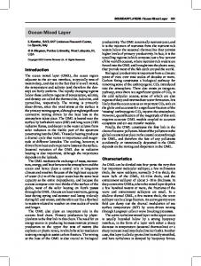
2-D and 3-D linear disturbances with an oblique wave angle of about 500 for the latter. The growth rate of the mass flow fluctuations (defined in Eqs. (28) and (29)) from our PSE calculations together with the multiple-scales results are plotted along with the growth rates obtained by quasi-parallel linear stability theory in Fig. 4. Our PSE results agree quite well with those obtained from the multiple-scales approach. The results also indicate that for the first mode disturbance at Mach 1.6, flow non-parallelism has more effect on three-dimensional disturbances than on two-dimensional ones. Results obtained at higher Mach numbers also show a noticeable non-parallel effect on the first-mode instability. We now show some results for the Mach 4.5 flat-plate flow, which is subject to second-mode instability (Mack 1984). Calculations were performed for a disturbance frequency of F = 1.2 x 10⁻⁴ with different streamwise resolutions. We used step sizes ranging anywhere from 64 steps per wavelength to only one step per wavelength. The results for the second-mode growth rate based upon the total kinetic energy are plotted in Figure 5. There is essentially no difference in the growth rate results when two or more steps per wavelength are used. The reason why only two points per wavelength could yield such accurate growth rates lies in the fact that most of the wave information is absorbed in the complex wavenumber a. In contrast, direct numerical simulation (DNS) of Navier-Stokes equations would require many more points per wavelength for comparable accuracy. To further verify our linear results, we compare non-parallel evolution of a second mode disturbance with a frequency of 2.2 x 10⁻⁴ with DNS. In Fig. 6, the maximum amplitudes of various flow quantities are plotted against Reynolds numbers for both PSE and DNS. The PSE results obtained by using only 7 steps per wave length agree very well with DNS results using 16 steps per wave length. The PSE calculation took about 100 seconds CPU time while the DNS required more than 40 hours on a Cray-YMP. Details of the comparison including nonlinear disturbances and the spatial DNS algorithm are given in Pruett and Chang (1993). Nonlinear PSE a. Computation of a In a previous section we mentioned that the wavenumber a for the harmonics may be determined either by the phase-locking rule or by using Eq. (17). It is known that the nonlinear wave interaction is dependent on the phase-difference between various modes. Therefore, it is essential that nonlinear PSE approach must not require phase-locking as a fundamental assumption; although, it may be used as a convenience for problems where phase-locking happens anyway. In order to demonstrate that phase-locking is not a basic assumption for nonlinear PSE computations, the following test has been performed. Nonlinear calculations have been done for a flat-plate boundary layer in the incompressible limit. A two-dimensional wave with a frequency F = .86 x 10' and an initial amplitude of 16
.25% at R = 400 is introduced in the boundary layer and the evolution of this wave along with its various harmonics is monitored. Calculations were performed in two different ways. First, the wavenumber a was computed for the fundamental wave according to Eq. (17) and the phase-locking rule was used for all the harmonics. In the second set of calculations, wavenumbers for the fundamental and all the harmonics were computed independently by using Eq. (17). The computed results for the amplitude of u velocity (fundamental, its four harmonics and meanflow correction) are presented in Fig. 7(a). It can be seen that only very minor differences appear between the two sets of calculations and these also tend to disappear as the calculations are marched away from the inflow boundary. The second set of calculations takes about 50% more computer time due to the iterations involved in determining a for the wave harmonics. Hence, it is expedient to use the phase-locking rule for problems where this may be the outcome in any case. In Fig. 7(b), the same nonlinear PSE results are compared with the spatial incompressible DNS results for fundamental, first harmonic and the mean flow distortion modes. Both PSE and DNS start with the same initial conditions, i.e., a fundamental disturbance (1, 0) at R = 400 and all harmonic waves including the mean flow distortion are generated through nonlinear interactions. The good agreement between DNS and nonlinear PSE indicates that the parabolizing approximation in the PSE approach does not introduce any severe error and all detailed nonlinear features are properly captured. Details of the comparison including disturbance profiles can be found in Joslin et al. (1992). b. Second-Mode Instability at Mach 4.5 To verify the nonlinear PSE algorithm, we choose the nonlinear second mode simulation at Mach 4.5 investigated by Erlebacher and Hussaini (1990) using the temporal DNS approach. As in the temporal DNS approach, we assume that the mean flow is parallel and study the spatial evolution of disturbances in the presence of nonlinear interactions. The initial conditions were provided by the eigensolution from the linear theory at R = 781 and four Fourier modes (M = 3) were kept in the truncated series. In our PSE calculation, the disturbance is assumed to be periodic in time and the nonlinear evolution is carried downstream in x as opposed to the temporal DNS approach where the disturbance is periodic in x and integration is carried in time. It was found in Erlebacher and Hussaini (1990) that due to nonlinear effect, the growth rate of the fundamental disturbance strongly depends on y and there exists a sharp decrease in the local growth rate near the critical layer. The growth rates based on ill 0 from our PSE results are shown in Figure 8(a) for different x locations. The growth rate is initially uniform at the starting location (x = OA). As the disturbances are evolving downstream, r.cnlinear effects observed in Erlebacher and Hussaini (1990) are evident in the present spatial calculations. For comparison, their temporal DNS results are shown in Figure 8(b) at different time levels represented as multiples of the temporal period r. Figure 9 depicts the amplitudes of the density fluctuation of the first harmonic for both PSE calcula17
tions and the DNS results. The DNS results in Figure 9 are re-scaled to facilitate comparison. Qualitatively, all nonlinear features observed in DNS, including the kink near the boundary-layer edge, are properly resolved in our PSE results. c. Subharmonic and Fundamental Resonance at Mach 1.6 Numerical simulation of incompressible flows have shown that the rapid growth of three-dimensional secondary disturbances is followed by breakdown to turbulence. Secondary instability is triggered when the primary disturbances reach sufficiently high amplitudes. To show the capability of the PSE approach in simulating transition onset, we also perform nonlinear calculations to study the secondary instability mechanism. We carry our calculations all the way to transition for both K-type (fundamental) and H-type (subharmonic) breakdown. We choose Mach 1.6 flat plate flow with a primary disturbance frequency of 0.5 x 10-. The same flow conditions were also used by Thumm et al. (1989) in their spatial Navier-Stokes simulations of a compressible boundary layer. We first perform a series of calculations to determine the amplitude of the primary disturbance which will trigger the secondary instability. The PSE calculation is initiated at a Reynolds number R of 460 where we impose a primary 2-D wave (mode (2, 0)) obtained by a local eigenvalue calculation and two subharmonic waves ((1, 1) and (1, -1) modes) by using the compressible secondary instability theory (Ng and Erlebacher, 1992) and all the remaining harmonics are assumed to have zero amplitudes. Initial amplitudes of the primary disturbances are set to be 3%, 1.1% and 0.6% at the inflow plane which corresponds to the 5%, 2% and 1% (the maximum amplitudes near the vibrating ribbon) cases given in Thumm et al. (1989). The initial amplitudes of the subharmonic waves are fixed at 0.019% for all three cases. The spanwise wave number of the subharmonic mode is fixed at 13/R = 0.53 x 10⁻⁴ which corresponds to an oblique wave angle of 450. Six temporal Fourier modes and three spanwise modes (M = 5 and N = 2) are kept in the Fourier series. The evolution of both primary and subharmonic disturbances are shown in Figure 10. Qualitatively, our results agree with those of Thumm et al.(1989). Any quantitative differences are due to different initial conditions. We find that a 1.1% initial amplitude (2% case in Thumm et al. (1989)) for the primary mode is enough to trigger the secondary growth; however, the onset of secondary growth for this case occurs at R = 800 where the primary wave is about to decay. We continue the PSE calculations beyond R = 1050 for this case and find that the secondary disturbance eventually saturates and the flow does not reach the transitional stage. To carry the 3% case to the transition stage, we made another calculation with more Fourier modes (M = 7 and N = 4) and the maximum velocity amplitudes of some representative modes are given in Figure 11. Besides the fundamental mode (2,0) and the subharmonic mode (1,1), higher harmonics in time and spanwise domain are also excited due to nonlinear interaction. Initially, the (4, 0) mode gains energy from self-interaction of the (2, 0) mode and the interaction of (2, 0) and (1, 1) produces the (3, 1) mode. When the subharmonic mode grows due to the onset of 18
secondary instability, its harmonic (2,2) also grows at slightly higher rate. The streamwise vortex mode (0,2) arises due to the interaction of (1, 1) mode and its complex conjugate (-1, 1). As all these modes continue to grow, more and more modes are excited. The energy cascade exhibits a staggered pattern. For instance, among the two-dimensional modes, only (2,0), (4,0), (6, 0), etc. gain energy; while for 1# modes, only (1, 1), (3,1), (5, 1), etc. are excited. The remaining modes (e.g. (1,0), (3,0), (0,1), (2, 1) etc.) remain unexcited throughout the calculation. The above staggered energy cascade is typical for subharmonic secondary instability. The secondary amplitude overtakes the primary at about R = 980 and reaches an equilibrium state around R = 1100. At this stage, many harmonic waves reach fairly high amplitudes as the flow heads for transition. We plot the time sequence of spanwise vorticity contours at the peak and valley planes (corresponding to the maximum and minimum disturbance rms amplitudes, respectively) in Figures 12(a) and 12(b). As can be seen, the vorticity pattern doubles its wavelength for x > 2200 (x is normalized w.r.t. the boundary layer length scale 1 at the initial plane) indicating the presence of high-amplitude subharmonic wave. It is also evident that the vortex roll-up results in a distinct kink in the shear layer. Towards the end of the computation, regions of intense vorticity near the wall begin to appear indicating that flow is heading for breakdown. Figure 13 shows the streamwise velocity contours in the x-z plane for a wall normal distance of y = 2.3, where the TS wave reaches its maximum according to the linear solution. The flow is initially two-dimensional and three-dimensional effect becomes important for x > 1800. For x > 2000, a staggered contour pattern is evident. This pattern is associated with the lambda vortex structure, a distinct characteristic of subharmonic breakdown, as observed in many incompressible experiments (e.g. Corke and Mangano (1989)). Nonlinear PSE calculations are also performed for the same Mach 1.6 case but for a fundamental-type secondary resonance. The initial amplitude of the primary wave is again 3% and that of the secondary is taken to be 0.005% to minimize nonlinear interaction close to the starting location. The spanwise wave number is O/R = 1.52 x 10⁻⁴ (oblique wave angle of 600 for the secondary wave) and the primary wave frequency is again 0.5 x 10⁻⁴. The initial conditions for our marching calculation consist of a 2-D primary wave (mode (1, 0)), two oblique fundamental-type secondary disturbances (mode (1, 1), (1, -1)) and the longitudinal vortex (mode (0, 1)). The same number of Fourier modes as in the subharmonic case is used. Nonlinear evolution of the maximum rms amplitude of u' is shown in Figure 14. Initially, the dominant modes are (1, 0), (1, 1), (0, 1) and (2, 0) (the first harmonic of the fundamental 2D mode). Unlike the subharmonic case, all harmonic waves (both odd and even modes) gain energy directly from nonlinear interaction. Among them, the (2, 1) (due to (1, 0) and (1, 1)) and (1, 2) (due to (0, 1) and (1, 1)) modes are more noticeable. For Reynolds numbers beyond 870, the spectrum is rapidly filled with high-amplitude disturbances and the flow is heading towards transition. As compared to the subharmonic breakdown, transition location shifts upstream due 19
to the larger growth rate of the secondary disturbance as a consequence of higher oblique wave angle. The time sequence of spanwise vorticity contours over a period of the primary wave is shown in Figures 15(a) and 15(b) for the peak and valley planes, respectively. In contrast to the subharmonic breakdoown, the wave length remains the same throughout the whole computational domain. One important characteristic of the K-type breakdown is the appearance of aligned lambda vortices. This is better visualized in the streamwise velocity contours shown in Figure 16 for x > 1300. Similar to that observed in incompressible simulations of Zang and Krist (1989), regions of intense shear begin to appear near the end of the computational domain in Figures 15(a) and 15(b). This indicates that flow has just entered the transitional stage. It is confirmed by plotting the average wall shear in Figure 17. The computed wall shear is slightly above the laminar value for most of the computational domain. Only towards the end, wall shear significantly departs from the laminar value indicating the onset of transition. In this way, PSE provides the prediction of boundary-layer transition for the imposed initial conditions. The PSE wall shear lies above the laminar value right from the beginning because of the relatively high amplitude of the 2-D primary disturbance needed for transition in supersonic flow. Since most amplified waves in supersonic flow are not two-dimensional, oblique primary modes may lead to transition for lower initial amplitudes. In order to carry the calculations further into transitional regime, more spanwise and temporal resolution will be required. It remains to be seen how far PSE can proceed into the transitional zone. The computational time used for the results presented in Figures 14-17 was 15 minutes on a Cray-YMP machine. Similar results from full compressible Navier-Stok-es equations would require 0(50) hours.
V. Conclusions Linear and nonlinear compressible boundary-layer stability is studied by using the PSE approach. Several issues concerning the characteristics of the parabolization and the updating of the streamnwise wave number are also discussed. The governing equations are solved by using second-order backward differences for the streamwise derivatives while the wall-normal direction is discretized by a fourthorder accurate finite- difference scheme. Non-parallel flow effects have been studied for linear disturbances. For oblique waves of the first mode type, the departure from the parallel results is more pronounced as compared to that for the two-dimensional waves. Our linear results are in good agreement with those from the multiple-scales approach, as well as those from full Navier-Stokes equations. Nonlinear PSE calculations are carried all the way to the early stage of transition for a Mach 1.6 flow. Both the subharmonic and fundamental types of break20
down are studied by the current PSE approach. Qualitatively, these breakdown processes are similar to the ones in incompressible boundary layers, except that high amplitudes of the 2-D primary wave are required. The promising results of our PSE calculations show that this new approach is a powerful tool for the study of boundary-layer stability and transition prediction. The parabolized form of the governing equations allow the numerical solution to be obtained in a computational time which is orders of magnitude lower than that required for direct simulation of Navier-Stokes equations.
References Bertolotti, F. P., Herbert, Th. and Spalart, P. R. 1992 "Linear and Nonlinear stability of the Blasius Boundary Layer," J. Fluid Mech., Vol. 242, pp. 4 4 1-4 74 . Chang, C.-L., Malik, M. R., and Hussaini, M. Y. 1990 "Effects of Shock on the Stability of Hypersonic Boundary Layers," AIAA Pdper No.90-1448. Chang, C.-L. and Merkle, C. L. 1989 "The Relation between Flux Vector Splitting and Parabolized Schemes," J. Computational Physics, Vol. 80, No. 2, pp. 344-361. Corke, T. C. and Mangano, R. A. 1989 "Resonant Growth of Three-dimensional Modes in Transitioning Blausius Boundary Layers," J. Fluid Mech., Vol. 209, pp.93150. Denier, J. P., Hall, P., and Seddougui, S. 0. 1991 "On the Receptivity Problem for G6rtler Vortices and Vortex Motions Induced by Wall Roughness," Phil. Trans. R. Soc. Lond. A, 335, pp.51-85. El-Hady, N. M. 1991 "Nonparallel Instability of Supersonic and Hypersonic Boundary Layers," Phys. Fluids A, Vol. 3, No.9, pp. 2164-2178. Erlebacher, G. and Hussaini, M. Y. 1990 "Numerical Experiments in Supersonic Boundary-Layer Stability," Phys. Fluids A, Vol.2 No.1, pp. 94 -1 0 4 . Gaponov, S. A. 1981 "The influence of Flow Non-Parallelism on Disturbance Development in the Supersonic Boundary Layers," Proceedings of the 8-th Canadian Congress of Applied Mechanics, pp. 673-674. Gaster, M. 1974 "On the Effects of Boundary-Layer Growth on Flow Stability," J. Fluid Mech., Vol. 66, pp.465-480. Hall, P. 1983 "The Linear Development of Girtler Vortices in Growing Boundary Layers," J. Fluid Mech., Vol. 130, pp. 4 1 -5 8 . Joslin, R. D., Streett. C. L. and Chang, C.-L. 1992 "Validation of ThreeDimensional Incompressible Spatial Direct Numerical Simulation Code - A Comparison with Linear Stability and Parabolic Stability Equation Theories for BoundaryLayer Transition on a Flat Plate," NASA Technical Paper TP-3205. Kachanov, Y. S. and Levchenko, V. Y. 1984 "The Resonant interaction of disturbances at Laminar-turbulent transition in a Boundary Layer," J. Fluid Mech., 21
Vol. 138, pp.209-247. Mack, L. M. 1969 "Boundary-layer Stability Theory," Document 900-277, Rev. A, JPL, Pasadena. Mack, L. M. 1984 "Boundary-Layer Linear Stability Theory," AGARD Report No. 709. Malik, M. R., Chuang, S., and Hussaini, M. Y. 1982 " Accurate Numerical Solution of Compressible, Linear Stability Equations," ZAMP, Vol. 33, 189. Malik, M. R. 1990a "Stability Theory for Laminar Flow Control Design," Viscous Drag Reduction in Boundary Layers, ed. D. M. Bushnell and J. N. Hefner, pp.3-46. Malik, M. R. 1990b "Numerical Methods for Hypersonic Boundary Layer Stability," J. Computational Physics, Vol. 86, No. 2, pp. 3 7 6 - 4 1 3 . Ng, L. and Erlebacher, G. 1992 "Secondary Instabilities in Compressible Boundary Layers", Phys. Fluids A, Vol. 4, No. 4, pp. 7 10 - 72 6 . Pruett, C. D. and Chang, C.-L. 1993 "A Comparison of PSE and DNS for HighSpeed Boundary-Layer Flows," ASME Fluids Engineering Conference, Washington, D. C., June 21-24, 1993. Rubin, S. G. 1981 "A Review of Marching Procedures for Parabolized NavierStokes Equations," Proceedings of Symposium on Numerical and Physical Aspects of Aerodynamic Flows, Springer-Verlag, New York, pp.171-186. Saric, W. S. and Nayfeh, A. H. 1975 "Non-parallel Stability of Boundary-Layer Flows," Phys. Fluids, Vol. 18. Spall, R. E. and Malik, M. R. 1989 "G6rtler Vortices in Supersonic and Hypersonic Boundary Layers," Phys. Fluids A, Vol. 1, No.11, pp. 1822-1835. Thumm, A, Wolz, W., and Fasel, H. 19?9 "Numerical Simulation of Spatially Growing Three-Dimensional Disturbance Waves in Compressible Boundary Layers," Proceedings of the third IUTAM Symposium on Laminar- Turbulent Transition, Toulouse, France, Sept. 11-15, 1989. Vigneron, Y. C., Rakich, J. V., and Tannehill, J. C. 1978 "Calculation of Supersonic Viscous Flow over Delta Wings with Sharp Subsonic Leading Edges," AIAA Paper No. 78-1337. Zang, T. A. and Krist, S. E. 1989 "Numerical Experiments on Stability and Transition in Plane Channel Flow," Theoretical & Comput. Fluid Dynamics, Vol. 1 No. 1, pp. 4 1 -6 4 .
22
/
v
-
0I C
0
/
/,
0
0) C> C
/1/
co
im
.o 0
00
C)~
0
0O
0
(0
C)
C)\L
o
0
C'J
o;
0
0 0
0
C0
0
0)
0 0D
231
0) 0) 0=
0 C 0
Co 0) Co
0
C)k
o)
a..
o0
b
co C~j
00 cl.4q:
Ec N-0 '!I! II
0
C)
0 $-4
0 00 C)
C>J o 0 0C
0 0 0 0
918
0 0 0 0
0 0 0 0
L41MOJE) IIoZ
24
1
a a 0)
0C0 0
0 0f
0
Oil0
E0
0
CDD
oO
4WX
CCfLO
I~ ole o2
WWW
!iIjE
C
II
0.0030
=0 0 ,50 0
4 M=1.6 F=0.4x 10V
F
--- a
0.0025
=500
0.00200.0015ry 0.00 10-
S/0.0005
0.0000-0.0005 -0.0010 II
I
I
600
800
I
I
1000
R Figure 4. Effect of non-parallel mean flows for both 2-D and 3-D disturbances of a Mach 1.6 flow at F = 0.4 x 10⁻⁴. (Solid lines are from parallel theory, dashed lines are from linear PSE calculations and results from El-Hady (1991) using the multiple-scales approach are shown by symbols).
26
1.00
co 0
C))
8L
0
1
o
CO
CC
U'j)1
LOO
C;
o2
Ii
0..e
II
(0mjE
8
0
Ii)
a:
t 0
LL
CTS*
0 0-
0
LLJ
0
.~J.
EpnlGow
U28
0 C\
C
V00
CCO
ob EC
00 C)
02
C
0
Ik
CLC .0 0
0
a
x0
coi 0
000
0 0
00
E
h
0
110
C
30
00
0 00 oo
.
-
4g
Co
4
4)
Ii
AR
I Iiz
Ii I
-
II
00
CO
0Y
0
o~C
00 0
0;
ejeld 41vo~JE .:
I
co
cl0
00
I I/-
co
C)
C)C
1
C)0
0;C
iC
~oE
eVl :3
0
.
"
0 0. 00 C.)) 0
0
0
91 -00
(1) 0
0
C.Cc -
Cu
0 C"'
C13
o0
o00
0
0
Aiisue] lo epnliidwV swi 33
00
0
0
4
d
x
I0
IN
LfI
0>
00
E
%-
0
00o.
If
C?
CDu
34
-
*
0)Qi%
i
oo
\
-o
ILL-
a)a o
0 CI
It
0 (
It
-9
It * II
I;
S
0
0
S
\0
.
0
0
35
0
.
20 15 y0 5 0
Mach 1.6 Subharmonic (peak plane) N0.0
0
20b0
x
2500
0 Y1 5 0 1 0
2C00
x
2500
x
250
1
20 15
2015 Y10 5
1200 20-20
t=0.6
15
--
... .... Y1 ..
5 0&A S200
x
2500
x
250o
20 15 Y10 5 01
15o200O
Figure 12. Time sequence of spanwise vorticity contours for the Mach 1.6 subharmonic breakdown (x and y are streamwise and wall-normal coordinates normalized by the boundary-layer length scale at R = 460): (a) Peak plane, (b) Valley plane. 36
20 15t=0
Mach 1.6 Subharmonic (valley plane)
Y1 5 20 15 Yb 5 200
x
2b
100200o
x
250o
10200o
x'
250o
10 20 15t=. 5 20 15t=. 5 20 15NO Y10 5
Fig. 12 (b)
37
Ifr)
C~j
c
1
0
0 0
ýt
-CD .2O
c
co_
_
:
_
_
_
_
_
E_
_
_
_
_
_
_
_
_
_
_
_
_
_
_
_
_
_
_
0
Z:, Dt
cN
0
0 0
co~
N
38
II C)
oor LL
a
0 00
LC 0
~O0
(U
CC
CDD 00
It I'
\
C'I Ci
39
' I6
\
hI
20 15 Y1
Mach 1.6 Fundamental (peak plane) t=0.0
5
05 0
7!0
1000
20 15
x 120
150
1500
t=0.2
ylO
5
0
05 0
760
1000
20 15 Y1 5 05
x 10
1500
150
1500
150
5b0
150
150
150
t=0.4
0
20 15 Y10 5 0 50
170
i
x 1250 t=0.6
70
1000
20 15
x 1250 t=0.8
5
0
5660
7t'0
1000
x'1250
Figure 15. Time sequence of spanwise vorticity contours for the Mach 1.6 fundamental breakdown : (a) Peak plane, (b) Valley plane. 40
20 15 YlO 5Ln 0 50
Mach 1.6 Fundamental (valley plane) t=0.0
70
100
20 15 ylO 0
x' 120
1530
1
t=0.2
1F0
5i070
20 15 YlO
X 125
50
170
t=0.4
5
20 00
7!0
100
Xl
0
150
150
1500
7 0
1506
150
20-
t=0.6
15 ylO0
5 0
50
70
10.0 x' 1ý50
20 15.
t=0.8
15 Ybb
5,0
"70
00
10x Fig.
150 15 (b)
41
LO
4)
4a
00
cd
V)V 0C\J
Cu
C."
N
)(42
Mach 1.6 Fundamental Breakdown 0.24 -
0.22
0.20 0 Q)
8 L 0.18 -
C-
Non-Linear PSE
0
Laminar
0.16-
N
0.14 IN
0.12 500
700 R
600
800
900
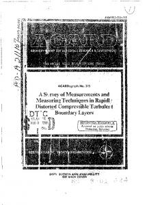
Figure 17. Wall shear of un-perturbed (laminar) and perturbed (PSE) flows versus Reynolds numbers for the fundamental breakdown shown in Figures 11 and 12.
43
REPORT DOCUMENTATION PAGE
F
orAAE-OW
wof th . searc"tO a nit g dVffaeta strtb~bad r~tn n ford etl;h.Jd udinghg flow,~t01 Ofe gather~~~~~~~~~~~~~~~~~nq~~~~ h aaneed n Oe~fgMdr~~l9tw(dt~ Ditftorrye fo 1 om 41n oon erif,.of Andftepofl. 1211ieffeno ine901 ftlet etcei. v to' "'I"C t'I" burdenl to We"Uqto" 6 nPlop" (0?04-OIUW),Watfurviton. DC 20103 R IM0. Athtlg=, VA 22024302, &Wto the office.of Mana qvont and 5~d.e PapWWremeot
m Collection OfInformation. including S4q to.0oS Damt Highwel. S~l I.
4.
-. REPORT TYPE AND DATES COVERED C) 93Cntr~tnrRavnnrt FUNDING NUMBERS
2. REPORT DATE
AGENCY USE ONLY (Lavaie biank)
ND
TTLE
UBTILE5.
LINEAR AND NONLINEAR PSE FOR COMPRESSIBLE BOUNDARY LAYERS
C NASI-18605 C NAS1-19480
AWHOR(S)WU
505-90-52-01
B. PERFORMING ORGANIZATION
7. PERFORMING ORGANIZATION NAME(S) AND ADDRESS(ES)
Institute for Computer Applications in Science and Engineering Mail Stop 132C, NASA Langley Research Center Hampton, VA 23681-0001
REPORT NUMBER
ICASE Report No. 93-70
10. SPONSORING/I MONITORING
2. SPONSORING / MONITORING AGENCY NAME(S) AND ADORESS(ES)
National Aeronautics and Space Administration Langley Research Center Hampton, VA 23681-0001
AGENCY REPORT NUMBER
NASA CR-191537 ICASE Report No. 93-70
III. SUPPLEMENTARY NOTES
Langley Technical Monitor: Final Report
Michael F. Card 12b. DISTRIBUTION CODE
12a. DISTRIBUTION /AVAILABILITY STATEMENT
Unclassified
-
UnlimitedI
Subject Category 341 13. ABSTRACT (Maximum200words) Compressible stability of growing boundary layers is studied
by numerically solving the partial differential equations under a parabolizing approximation. The resulting parabolized stability equations (PSE) account for nonparallel as well as nonlinear effects. Evolution of disturbances in compressible flat-plate boundary layers are studied for freestream Mach numbers ranging from 0 to 4.5. Results indicate that the effect of boundary-layer growth is important for linear disturbances. Nonlinear calculations are performed for various Mach numbers. Two-dimensional nonlinear results using the PSE approach agree well with those from direct numerical simulations using the full Navier-Stokes equations while the required computational time is less by an order of magnitude. Spatial simulations usin PSE have been carried out for both the fundamental and subharmonic type breakdown for a Mach 1.6 boundary layer. The promi3ing results obtained in this study show that the PSE method is a powerful tool for studying boundary-layer instabilities and for predicting transition over a wide range of Mach numbers.
14. SUBJECT TERMS
IS. NUMBER OF PAGES
stability, compressible, boundary layer, PSE
47 16. PRICE CODE
17. SECURITY CLASSIFICATION
OF REPORT Unclassified
I
I
1B. SECURITY CLASSIFICATION
OF THIS PAGE Unclassified
I OF ABSTRACT I__________ 19. SECURITY CLASSIFICATION
NSN 7540-01-2810-5500
20. LIMITATION OF ABSTRACT
Standard Form 298 (Rev 2-119) * U.S. GOVERNMENT PRINTING OMCE: 1993 - 52U-O4Itj&7l
Prewnded by ASIV Sid Zil-IS 2W6-02