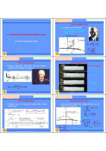
2. Overview. • Drag. • The boundary-layer concept. • Laminar boundary-layers. •
Turbulent boundary-layers. • Flow separation.
Lecture 11 – Boundary Layers and Separation Applied Computational Fluid Dynamics Instructor: André Bakker
http://www.bakker.org © André Bakker (2002-2006) © Fluent Inc. (2002)
1
Overview • • • • •
Drag. The boundary-layer concept. Laminar boundary-layers. Turbulent boundary-layers. Flow separation.
2
The drag force • The surrounding fluid exerts pressure forces and viscous forces on an object. τw
p0
• The components of the resultant force acting on the object immersed in the fluid are the drag force and the lift force. • The drag force acts in the direction of the motion of the fluid relative to the object. • The lift force acts normal to the flow direction. • Both are influenced by the size and shape of the object and the Reynolds number of the flow.
3
Drag prediction • The drag force is due to the pressure and shear forces acting on the surface of the object. • The tangential shear stresses acting on the object produce friction drag (or viscous drag). Friction drag is dominant in flow past a flat plate and is given by the surface shear stress times the area: Fd ,viscous = A.τ w • Pressure or form drag results from variations in the the normal pressure around the object: Fd , pressure = ∫ p dan A • In order to predict the drag on an object correctly, we need to correctly predict the pressure field and the surface shear stress. • This, in turn, requires correct treatment and prediction of boundary layers and flow separation. • We will discuss both in this lecture. 4
Viscous boundary layer • • • • • • • •
An originally laminar flow is affected by the presence of the walls. Flow over flat plate is visualized by introducing bubbles that follow the local fluid velocity. Most of the flow is unaffected by the presence of the plate. However, in the region closest to the wall, the velocity decreases to zero. The flow away from the walls can be treated as inviscid, and can sometimes be approximated as potential flow. The region near the wall where the viscous forces are of the same order as the inertial forces is termed the boundary layer. The distance over which the viscous forces have an effect is termed the boundary layer thickness. The thickness is a function of the ratio between the inertial forces and the viscous forces, i.e. the Reynolds number. As Re increases, the thickness decreases. 5
Effect of viscosity • The layers closer to the wall start moving right away due to the no-slip boundary condition. The layers farther away from the wall start moving later. • The distance from the wall that is affected by the motion is also called the viscous diffusion length. This distance increases as time goes on. • The experiment shown on the left is performed with a higher viscosity fluid (100 mPa.s). On the right, a lower viscosity fluid (10 mPa.s) is shown.
6
Moving plate boundary layer • An impulsively started plate in a stagnant fluid. • When the wall in contact with the still fluid suddenly starts to move, the layers of fluid close to the wall are dragged along while the layers farther away from the wall move with a lower velocity. • The viscous layer develops as a result of the no-slip boundary condition at the wall.
7
Viscous boundary layer thickness • Exact equations for the velocity profile in the viscous boundary layer were derived by Stokes in 1881. • Start with the Navier-Stokes equation: ∂u ∂ 2u =ν 2 ∂t
∂y
• Derive exact solution for the velocity profile: y U = U 0 1 − erf 2 ν t 2
z
• erf is the error function: erf ( z) = π ∫ e dt • The boundary layer thickness can be approximated by: −t 2
0
∂u ∂ 2u U U = ν 2 ⇒ 0 ≈ ν 20 ⇒ δ ≈ ν t t δ ∂t ∂y 8
Flow separation • Flow separation occurs when: – the velocity at the wall is zero or negative and an inflection point exists in the velocity profile, – and a positive or adverse pressure gradient occurs in the direction of flow.
9
Separation at sharp corners • Corners, sharp turns and high angles of attack all represent sharply decelerating flow situations where the loss in energy in the boundary layer ends up leading to separation. • Here we see how the boundary layer flow is unable to follow the turn in the sharp corner (which would require a very rapid acceleration), causing separation at the edge and recirculation in the aft region of the backward facing step.
10
Flow around a truck • Flow over non-streamlined bodies such as trucks leads to considerable drag due to recirculation and separation zones. • A recirculation zone is clear on the back of the cab, and another one around the edge of the trailer box. • The addition of air shields to the cab roof ahead of the trailer helps organize the flow around the trailer and minimize losses, reducing drag by up to 10-15%.
11
Flow separation in a diffuser with a large angle
12
Inviscid flow around a cylinder • The origins of the flow separation from a surface are associated with the pressure gradients impressed on the boundary layer by the external flow. • The image shows the predictions of inviscid, irrotational flow around a cylinder, with the arrows representing velocity and the color map representing pressure. • The flow decelerates and stagnates upstream of the cylinder (high pressure zone). • It then accelerates to the top of the cylinder (lowest pressure).
• Next it must decelerate against a high pressure at the rear stagnation point. 13
Drag on a smooth circular cylinder • The drag coefficient is defined as follows: Fdrag = C D 12 ρ v 2 A⊥
no separation steady separation unsteady vortex shedding laminar BL wide turbulent wake
turbulent BL narrow turbulent wake 14
Drag on a smooth circular cylinder • At low Reynolds numbers (Re < 1), the inertia effects are small relative to the viscous and pressure forces. In this flow regime the drag coefficient varies inversely with the Reynolds number. For example, the drag coefficient CD for a sphere is equal to 24/Re.
no separation
15
Drag on a smooth circular cylinder • At moderate Reynolds numbers (1