1 INSA Lyon, GEMPPM Laboratory, 20, Ave Albert Einstein, 63621 Villeurbanne Cedex and. Lafarge ...... http://ciks.cbt.nist.gov/monograph part I, ch 6, section 8.
INSTITUTE OF PHYSICS PUBLISHING
MODELLING AND SIMULATION IN MATERIALS SCIENCE AND ENGINEERING
Modelling Simul. Mater. Sci. Eng. 9 (2001) 371–390
PII: S0965-0393(01)25823-9
Linear elastic properties of 2D and 3D models of porous materials made from elongated objects S Meille1 and E J Garboczi2 1 INSA Lyon, GEMPPM Laboratory, 20, Ave Albert Einstein, 63621 Villeurbanne Cedex and Lafarge LCR, 95, rue du Montmurier, BP 15, 38 291 St Quentin Fallavier Cedex, France 2 National Institute of Standards and Technology, Building Materials Division, 100 Bureau Drive Stop 8621, Gaithersburg, MD 20878-8621, USA
Received 12 March 2001, accepted for publication 29 May 2001 Published 17 July 2001 Online at stacks.iop.org/MSMSE/9/371 Abstract Porous materials are formed in nature and by man by many different processes. The nature of the pore space, which is usually the space left over as the solid backbone forms, is often controlled by the morphology of the solid backbone. In particular, sometimes the backbone is made from the random deposition of elongated crystals, which makes analytical techniques particularly difficult to apply. This paper discusses simple two- and three-dimensional porous models in which the solid backbone is formed by different random arrangements of elongated solid objects (bars/crystals). We use a general purpose elastic finite element routine designed for use on images of random porous composite materials to study the linear elastic properties of these models. Both Young’s modulus and Poisson’s ratio depend on the porosity and the morphology of the pore space, as well as on the properties of the individual solid phases. The models are random digital image models, so that the effects of statistical fluctuation, finite size effect and digital resolution error must be carefully quantified. It is shown how to average the numerical results over random crystal orientation properly. The relations between two and three dimensions are also explored, as most microstructural information comes from two-dimensional images, while most real materials and experiments are three dimensional.
1. Introduction The processes that are used to form natural and man-made porous materials are diverse. Some are formed by introducing bubbles into a viscous liquid, then hardening the liquid, as in foaming processes. However, many porous materials are formed by building up a solid structure that incorporates empty areas into its overall body. In this case, the morphology of the pores, which are made from the ‘left-over’ space around the forming solid backbone, is mainly determined by the morphology of the solid products. This is the case for cement-based 0965-0393/01/050371+20$30.00
© 2001 IOP Publishing Ltd
Printed in the UK
371
372
S Meille and E J Garboczi
materials, which are among the most highly-used porous materials produced by mankind. One particular kind of cement-based material is gypsum plaster, widely used for the production of gypsum plaster board, of which billions of square metres are produced every year across the world. This material is an example of a porous solid made up from elongated gypsum crystals that randomly intersect and grow together from seeds to form a random porous solid. In general, there has been some success in using bounds, expansions and effective medium theories to understand the effective properties of composite materials made up from inclusions in a matrix [1, 2]. However, these analytical theories have not, in general, been terribly successful in describing the effective properties of microstructures made up from intersecting solid objects and particularly elongated objects. Hence the need to turn to simple computer simulation models to help sort out these relationships. Chapter 1 in [3] describes a ‘tool-kit’ of computational methods that can be used to analyse digital images of porous materials. One part of this collection of tools is a suite of finite element programs that can be used to explore many aspects of the linear elastic properties of random porous materials [4]. These can be used to explore quickly many different random models of random porous media, examining their effective elastic properties as a function of porosity and pore morphology. These numerical data can then be used to interpret and explain experimental data. This paper is then a computational investigation of the linear elastic properties of various simple models for random porous materials made up from the random arrangement of solid elongated objects (bars). We investigate how the morphology of the solid and pore space affects the elastic properties, and how varying the solid properties affects the overall elastic properties. Comparisons between two dimensions (2D) and three dimensions (3D) are especially useful, because most microstructural information is obtained in 2D, from images of various kinds, while the measurement of elastic properties is in 3D. Also, because these are random digital models, the effects of statistical fluctuation, finite size effect and digital resolution errors must be carefully quantified in order to ensure valid results. Comparison is made both with the elastic properties of other random models, and to measured elastic properties of real materials. The emphasis of this paper is on how solid and pore morphology affect elastic properties, and on how simple models can be used to help elucidate the phenomena found in real porous materials. 2. Models and elastic techniques We give here a brief description of the models used, and the motivation for using them, along with a short description of the finite element technique used to solve for the effective elastic moduli in 2D or 3D. 2.1. Models The basic unit of all the models to be described in this paper is the bar, which is a rectangle in 2D and a rectangular parallelepiped in 3D. The aspect ratios of the bars were taken to be 7:1, roughly based on average values found in experiments on porous gypsum plasters and on numerical considerations—the size of the unit cell needed to be about five to ten times larger than the longest dimension of the bars, so too high an aspect ratio would have meant too large a unit cell for reasonable computational turnaround rates of the many results required. These bars were taken to be totally solid, and were placed randomly in several ways in a periodic unit cell. By ‘periodic’, we mean that if a bar extended past the side of the unit cell, it was completed periodically on the other side of the cell. The pore space was then the space in the unit cell not occupied by the solid.
Linear elastic properties of models of porous materials
373
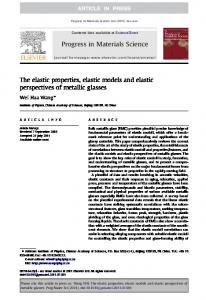
In 2D and 3D, the first type of model to be studied were built by randomly placing the centre of the bars, and allowing the bars to be oriented in one of the principal directions (x, y in 2D and x, y, z in 3D) (O-HV). Figure 1(a) shows an example of this arrangement in 2D. When the system size was 2002 , the typical size used in the 2D studies, the bars were 21 × 3 pixels in size. In 3D, the bars were 21 × 3 × 3 pixels in dimension when the system size was 1003 . In 3D, a model where the bars were allowed to have random orientations was also briefly studied (O-R). Another type of model was generated by first randomly placing bars in the principal directions (these were not allowed to overlap (hard cores)), and then by expanding each bar around its centre through adding a ‘soft shell’ that could freely overlap both phases. The hard cores were placed with random jamming statistics [5, 6]. This model version was inspired by the ‘hard core/soft shell’ model usually used with spheres and ellipsoids and is denoted in the text as HCSS-HV [5, 6]. Figure 1(b) shows an example of this type of model in 2D. In 2D, at a system size of 2002 pixels, the hard core was a 19 × 1 pixel rectangle, and the soft shell was 1 pixel in width, so that the total size of the complete object was the same as for the O-HV case. Similarly, in 3D, at a system size of 1003 pixels, the hard core was 19 × 1 × 1, with a 1 pixel thick soft shell.
(a)
(b)
Figure 1. Models used in the 2D computations (2002 pixels): (a) O-HV and (b) HCSS-HV. Dark grey = pore, medium grey = unoverlapped solid, white = overlapped solid regions. Phase fractions are: (a) 27.7% porosity, 37% non-overlapped solid, and 35.3% overlapped solid; (b) 21.8% porosity, 39.7% non-overlapped solid, and 38.5% overlapped solid.
We note here that having a model in which the microstructure is split into individual pixels gives the model great flexibility. For example, it is simple to monitor the percolation quantities of both the solid and pore phases using a burning algorithm [4, 7]. In addition, to calculate the overlap volume between two ellipsoids is a fairly formidable mathematical problem. To analytically calculate the overlap between three or more ellipsoids is almost impossible. But in a digital model, it is easy to keep track of how many bars have been placed on the same pixel, so the total overlap area (2D) or volume (3D) can be readily known. Figure 2 shows the overlap solid fraction versus the porosity for the two different 2D models. The 2D HCSS-HV model has somewhat less overlap area at a given porosity than the O-HV model does. This is because the hard core regions cannot overlap one another, while in the O-HV model, all pixels have the potential of participating in the overlaps. The overlap fraction was investigated as a function of size of the system and digital resolution, and was found to give reasonable results at the typical sizes used in 2D.
374
S Meille and E J Garboczi 0.8
Overlap fraction
0.7 0.6 O - HV 0.5
HCSS - HV
0.4 0.3 0.2 0.1 0 0
0.2
0.4
0.6
0.8
Porosity
Figure 2. Variation of overlap fraction versus porosity fraction for the 2D models described in figure 1.
2.2. Elastic moduli equations and numerical techniques Since the elastic properties of both 2D and 3D models will be computed in this paper, it is important to write down both sets of elastic properties and indicate the relationship between them. The following discussion is taken from [8]. Hooke’s law for an isotropic 3D body, which defines the elastic moduli, is: εxx = (1/E3 )[σxx − ν3 (σyy + σzz )]
εxy = [(1 + ν3 )/E3 ]σxy
(1)
along with cyclic permutations of x, y and z. Young’s modulus is E and Poisson’s ratio is ν. Simply writing Hooke’s law for an isotropic 2D body results in εxx = (1/E2 )[σxx − ν2 σyy ]
εxy = [(1 + ν2 )/E2 ]σxy
(2)
along with cyclic permutation of x and y. The subscripts on the moduli indicate the dimension in which they are defined. The relationships between the various isotropic moduli for 3D are 9 1 3 3K3 − 2G3 = + υ3 = E3 K3 G3 2(3K3 + G3 ) K3 = E3 /[3(1 − 2ν3 )] G3 = E3 /[2(1 + ν3 )]
(3)
4 1 1 K2 − G 2 = + υ2 = E2 K2 G 2 K2 + G 2 K2 = E2 /[2(1 − ν2 )] G2 = E2 /[2(1 + ν2 )].
(4)
and for 2D are
Note that for K (bulk modulus) and G (shear modulus) to be non-negative, and so give a stable elastic system, the bounds on Poisson’s ratio are −1 < υ3 < 1/2 (3D) −1 < υ3 < 1 (2D).
(5)
Torquato [9] has written equivalent relations between the various isotropic elastic moduli for general dimensions in his recent book on the theory of composite materials. We can relate 3D to 2D moduli if we assume that the 2D equations have been derived from the 3D equations via
Linear elastic properties of models of porous materials
375
the assumption of plane strain (all out-of-the-plane strains are zero) or plane stress (all out-ofthe-plane stresses are zero). If we make the plane strain assumption, then the 3D equations transform to the equivalent of the 2D equations, with the mapping E3 ν3 E2 = . (6) ν2 = 2 (1 − ν3 ) (1 − ν3 ) If we make the assumption of plane stress, then the same thing happens again, but with the new mapping E2 = E3
ν2 = ν3
(7)
which, interestingly enough, makes the 2D and the 3D moduli numerically equal to each other but with different units. The finite element technique (in FORTRAN 77) used to solve the elastic equations has been thoroughly described [10], and a manual covering details of the theory and usage has been written [4]. Briefly, each pixel is treated as a finite element, so that the finite element mesh is just the lattice of the digital image itself. The continuum elastic equations can be solved exactly via a variational principle, where the correct solution is found by minimizing the elastic energy stored in the material, given the constraint of the applied strain. The finite element technique minimizes the digital elastic energy, so that the best solution, given the discretization of the problem, is found. The elastic displacements are found in every pixel, and the average strain and stress in each pixel is computed and averaged over the entire microstructure to give the effective elastic properties of the porous material. The memory required to run these models is about 150 byte per pixel, in 2D, and about 230 byte per pixel in 3D. The total memory required for two typical systems used, 2002 in 2D and 1003 in 3D, then required, respectively, 6 and 230 Mbyte. Obviously, much larger systems can be studied in 2D. In 3D, somewhat larger systems can be studied, although the memory required quickly reaches the multi-gigabyte range. Run times will vary with the computer used. The materials we are trying to simulate are elastically isotropic random collections of overlapping, elongated crystals. In analysing the elastic properties of the models, we want to achieve isotropic moduli, as this is what is measured. But when bars are placed only in the principal directions, then the effective elastic moduli are not isotropic. In addition, they do not even have square (2D) or cubic (3D) properties, because of their randomness. There are then two types of averaging that must be done. The first is averaging over random configurations, because of statistical fluctuation, which is described in the next section. The second is angular averaging. In the following, we describe an averaging technique that results in isotropic elastic moduli. Consider the 3D case first. The elastic moduli tensor obtained for one configuration of a given model cannot be assumed to follow any particular crystal pattern. In Voigt notation, a general symmetric 6 × 6 matrix, with 21 independent elements, has the following form: C11 C12 C13 C14 C15 C16 C12 C22 C23 C24 C25 C26 C23 C33 C34 C35 C36 C Cij kl = 13 (8) C14 C24 C34 C44 C45 C46 C15 C25 C35 C45 C55 C56 C16 C26 C36 C46 C56 C66 where 1 = xx, 2 = yy, 3 = zz, 4 = xz, 5 = yz, and 6 = xy. The tensor in 2D, with six independent elements, has the form: � � C11 C12 C16 Cij kl = C12 C22 C26 (9) C16 C26 C36
376
S Meille and E J Garboczi
where 1 = xx, 2 = yy, and 6 = xy (we use ‘six’ instead of the more natural ‘three,’ in order to link more clearly to 3D). The computed elastic tensor of one of the 3D models will, in general, have the symmetry of equation (8). We can analytically average this tensor, using the full Cij kl form of the elastic moduli tensor, over the three Euler angles (α, β, γ ) in 3D and the single polar angle (φ) in 2D. The 3D Euler angle matrix is [11]: � � cos γ cos β cos α − sin γ sin α cos γ cos β sin α + sin γ cos α − cos γ sin β Aij = − sin γ cos β cos α − cos γ sin α − sin γ cos β sin α + cos γ cos α sin γ sin β . sin β cos α sin β sin α cos β (10) The 3D equation for angularly averaging the elastic moduli tensor is then [11]:
2π
π
2π 1 C dα sin β dβ dγ Ami Anj Apk Aql (11) �C�ij kl = mnpq 8π 2 mnpq 0 0 0 where Cmnpq is a constant, evaluated in some set of Cartesian axes. This will result in an isotropic tensor, with the values of K and G given by �C11 � = 15 (C11 + C22 + C33 ) + G=
1 [(C11 15
K = �C11 � −
2 (C12 15
+ C13 + C23 )
+ C22 + C33 ) − (C12 + C13 + C23 ) + 3(C44 + C55 + C66 )]
(12)
4 G. 3
Note that the ij terms where i = 1, 2, 3 and j = 4, 5, 6, and vice versa, do not appear in the averages. This leads us to formulate a simpler averaging process, where the angular averaging process need not be used explicitly. Define an average cubic material with cubic symmetry in 3D, so that there are three independent elastic moduli: (C11 )avg , (C12 )avg and (C44 )avg , defined in the following straightforward way: (C11 )avg = 13 (C11 + C22 + C33 ) (C44 )avg = 13 (C44 + C55 + C66 ) (C12 )avg =
1 (C12 3
(13)
+ C13 + C23 ).
The fully angularly averaged equations (12) then become: �C11 � = 35 (C11 )avg + 25 (C12 )avg G = 15 [(C11 )avg − (C12 )avg + 3(C44 )avg ] K = �C11 � −
(14)
4 G. 3
Equations (14) look like the equations obtained when angularly averaging a cubic elastic moduli tensor [12], with (C11 )avg → C11 , (C44 )avg → C44 and (C12 )avg → C12 , the three independent elements of a cubic elastic moduli tensor. The relevant rotation matrix in 2D is: � cos φ sin φ Aij = . (15) − sin φ cos φ The same averaging procedure can be done in 2D [11], according to
2π 1 Cmnpq dφAmi Anj Apk Aql �C�ij kl = 2π mnpq 0
(16)
Linear elastic properties of models of porous materials
377
with the results �C11 � = 18 (3C11 + 3C22 + 2C12 + 4C66 ) G = �C66 � = 18 (C11 + C22 − 2C12 + 4C66 ) K = �C11 � − G.
(17)
If we define (C11 )avg = 21 (C11 +C22 ), then equations (17) become the equations for an effective square symmetry elastic moduli tensor [12]: K = �C11 � − G �C11 � = 41 [3(C11 )avg + C12 + 2C66 ] G = �C66 � =
1 [(C11 )avg 4
(18)
− C12 + 2C66 ].
If the bars were oriented randomly in all directions, then the effective moduli would not need to be rotationally averaged, but just averaged over different configurations. However, for a nominally isotropic random system, a rotational average should be very similar to a configurational average. Note that since equations (11) and (16) are linear in Cmnpq , the configurational average and the rotational average can be taken in any order. In summary, the ‘experimental’ technique is as follows: build a microstructure using one of the previous rules and a random number generator, assign elastic properties to the solid phase(s), and use the programs to compute the effective elastic moduli of the model. To obtain all 21 of the elements in equation (8), six runs must be made for each system considered, with only one of the six independent strains (ε1 , ε2 , ε3 , ε4 , ε5 , ε6 ) non-zero each time. Using the average stress tensor, �σij �, we can then define the effective elastic tensor by �σij � ≡ �Cij kl �εij , where εij is the applied strain. Using this technique, all 21 elements can be evaluated. The symmetry of the tensor is then a check of the numerical technique, as elasticity theory requires that the elastic moduli be symmetric for infinite systems. Using periodic boundary conditions in this case gives an effectively infinite system, as there is no surface. This general symmetry elastic moduli tensor should then be angularly averaged to produce isotropic elastic moduli. In the next section, we discuss how solid moduli were picked, and how to analyse the sources of error in this process. 3. Solid elastic moduli and error analysis 3.1. Solid elastic moduli One of our interests, as discussed in the introduction, is in porous materials such as cementbased materials and, in particular, gypsum plaster. Therefore, we chose to use the measured elastic moduli of gypsum crystals for the solid backbone moduli. If the backbone moduli tensor is isotropic, then the Young’s modulus E of the porous composite will scale with the magnitude of Es . The shape of the E/Es versus porosity graph, for an isotropic backbone, will not depend at all on the value of νs in 2D [8] and only mildly so in 3D [2]. However, since gypsum plaster is the material that we are looking to model, we have to deal with the gypsum crystal elastic moduli tensor, which is not isotropic. The gypsum crystal has monoclinic symmetry, so that its 3D elastic moduli tensor contains 13 independent constants. The measurement of these constants using an acoustic method has been published [13]. As the crystal anisotropy would be very difficult to handle computationally when the crystals are overlapping, and also because we are ultimately interested in real porous materials, which are usually isotropic, we will make the assumption of an isotropic tensor for the solid
378
S Meille and E J Garboczi
backbone. An angular average, using equation (11) with the full gypsum elastic moduli tensor, leads to [14] Ks = 44 GPa
Gs = 17 GPa
(19)
The corresponding values of Young’s modulus E and Poisson’s ratio ν are: Es = 45.7 GPa
νs = 0.33.
(20)
Equations (19) and (20) are the isotropic average of the 3D tensor. If we want to study 2D models, a 2D equivalent must be found. As discussed in section 2.1, there are two choices for making 2D moduli from the 3D moduli: plane strain or plane stress. The plane-strain values of Young’s modulus and Poisson’s ratio are: Es = 50 GPa, νs = 0.45. For all the 2D studies, the plane-strain values of the 2D moduli were used. The plane-stress values were used in the data to be presented in figure 12 in section 5. 3.2. Error analysis In any microstructure model of a random material, there are always two sources of error: statistical fluctuation and finite size effect [1, 15]. The first comes about because when constructing a model, there are many different choices for the random numbers possible that determine the arrangement of the phases. Each choice, in principle, can have different properties. This sensitivity to statistical fluctuation must be carefully tested. The second source of error, finite size effect, comes about because the unit cell of the model can only contain a piece of the microstructure that is small compared to a experimental piece of the real material. One must ask the question: is the model big enough so that its microstructure is typical of the real material [16, 17]? In digital models, there is a third source of error: digital resolution. Arbitrary shapes are being represented by a collection of square or cubic pixels, and there will almost always be a dependence of properties on resolution. This can come about in two ways. Suppose we compute the properties of a composite made up of cubical particles that are randomly placed but oriented with the digital pixel axes. In this case, the shape of the particles is always represented properly, but the continuum elastic equations are discretized, so that the resolution will still have an effect. If the particles were spheres, or cubes or bars that were not aligned with the digital pixel axes, the shape of the particles would then also change with resolution, adding to the digital resolution error. These sources of uncertainties will be discussed as we analyse the results of each model in the following section. 4. Results 4.1. Two-dimensional model results Figure 3 shows how the digital resolution error is dealt with for the O-HV model. The elastic moduli were computed at different resolutions and then plotted against the reciprocal of the number of pixels per side of the unit cell, 1/N . For example, if 600 21 × 3 bars were used to construct a 200 × 200 pixel unit cell system, then to double the resolution, the same number of 42 × 6 bars would be used for a 400 × 400 pixel unit cell system. The value of C11 is shown in figure 3, as it was typical of all the other elastic moduli. The result found previously was that in the large N limit, where ‘large’ is different for different models, the moduli scale like 1/N [15, 18]. By extrapolating to the N = ∞ limit (1/N = 0), the true value for infinite resolution can be accurately approximated. This procedure has been checked for a single sphere in a matrix, where the true value is known [19], and was found to be accurate.
Linear elastic properties of models of porous materials
379
40 35
C 11 (GPa)
30 25 13 % porosity 36 % porosity 45 % porosity
20 15 10 5 0 0
0.001
0.002
0.003
0.004
0.005
1/N
Figure 3. Resolution influence on the value of C11 for the 2D O-HV model, at different porosity fractions. The three system sizes are (N 2 in pixels) 2002 , 4002 and 10002 pixels.
The three lines on figure 3, for the three different porosities, seem to be similar. However, if we examine the percentage difference between the 2002 system values and the infinite limit extrapolated values, we find that this difference depends roughly linearly on the porosity (10% at the lowest porosity and about 40% at the highest porosity). This is not hard to understand. If the porosity were zero, extrapolation would make no difference at all, as the solid elastic moduli would be replicated exactly in each solid pixel. Even one pixel, representing the entire system, would give the correct elastic moduli. As porosity increases, the model becomes increasingly random, with more intricate morphology, so that more and more resolution is needed to represent correctly complex shapes and compute the elastic properties. This was found to be true for the 3D models as well. All the 2D models considered had similar asymptotic behaviour. Since in 2D, we were mainly interested in comparisons between the different microstructures, only non-extrapolated results were used, in order to save computational time. The extrapolated results are used later in the paper when comparing 3D model results to experimental data, since extrapolation did make a significant difference in the computed quantities. In all the models considered in this paper, errors due to the finite size effect and statistical fluctuation were much less than the error induced by digital resolution. When reasonably far away from the percolation threshold in any model, 2D or 3D, it was found adequate to use only one realization of each model, as these errors were only on the order of 1–2%. However, near the percolation threshold, the statistical fluctuation and finite size effect errors increased greatly. Since we are not very interested in behaviour near the percolation threshold, at least not in this paper, there was no additional averaging to obtain less uncertain results in this regime. Consequently, the details of the elastic behaviour near the percolation threshold have associated large error bars (not shown on the graphs). Figure 4(a) shows Young’s modulus (isotropically averaged for the HV models) of the two different 2D models, plotted against porosity. Note that the HCSS models tend to be somewhat less stiff than the overlapping models. Comparing figure 4(a) with figure 2, we can see that at a given porosity, there is more overlap area for the overlapping models than for the HCSS models. Since this overlap area is what gives the models their stiffness, more overlap area translates to higher stiffness at the same porosity. Also, going along with this fact, the percolation thresholds for the models are different. The percolation threshold, which is the porosity at which the solid phase becomes geometrically disconnected, is somewhat higher for
380
S Meille and E J Garboczi
the O-HV model (about 0.6) than for the HCSS-HV model (0.45). This implies that at a given porosity, where both models are still percolated, the O-HV model will be better connected than the HCSS-HV model, causing it to be stiffer. This ‘better connectedness’ is also clearly correlated closely with the overlap fraction (figure 2). Figure 4(b) shows Poisson’s ratio for the 2D models plotted against porosity. Similar behaviour is seen for both models. The solid Poisson ratio, 0.45, may seem high, but note that equation (5) allows values of ν in 2D up to one, when the allowable maximum in 3D is only 1 . Adding porosity seems to lower the effective Poisson ratio. As is known in 2D exactly, 2 Poisson’s ratio tends to flow towards a fixed point, as the percolation threshold is approached. The data shown in figure 4(b) then imply that for both models, the value of this fixed point is between 0.2 and 0.3. The large uncertainties in the data near the percolation threshold do not allow a more specific statement to be made. If, however, the fixed point was to be 0.45 or higher, then adding porosity would make the Poisson ratios increase with increasing porosity. We shall see an example of this type of behaviour in 3D. Figure 5 shows an interesting example of what was briefly touched on in section 2: the flexibility of digital models. For the O-HV and HCSS-HV models, the overlap area was separately labelled from the other solid parts, and allowed to have a Young’s modulus different from the other parts of the solid backbone. This value was only allowed to be less than that of the bulk crystal backbone, as larger values were thought to be unphysical. The Poisson ratio remained the same, however. Both systems had a porosity of 27%. The overlap fractions, defined as the percentage of solid material that belongs to two or more bars, is 35% for the O-HV model and 31% for the HCSS-HV model. In figure 5, the overall Young’s modulus of each model, normalized by Young’s modulus when all solid parts had the same moduli (given for the two sets of data in figure 4(a), 27% porosity), is plotted against the fraction (less than one) of Eo /Eno for the solid phases (o = overlap, no = non-overlap). Because of the different normalizations for each model, the two sets of data overlap at unity when the ratio Eo /Eno = 1. It is interesting to note that the two models both now fall on nearly the same curve, as opposed to figure 4(a). Figure 5 shows a different kind of dependence on microstructure than figure 4(a) does, but the two graphs are not expected to be similar. We should note that there is another method used for computing the effective elastic moduli of porous materials based on a finite difference scheme [20]. This works well on uniform solid phases, but is very difficult to implement when there is more than one solid phase with different elastic properties. For example, the computational results shown in figure 5 would have been very difficult to obtain using this method. Also, the finite element technique [4, 10] can handle any symmetry elastic moduli tensor, which is possible but difficult in the finite difference technique [20].
4.2. Three-dimensional model results In figure 6 3D views of the three 3D models studied are shown: O-HV (figure 6(a)), HCSSHV (figure 6(b)), and O-R (figure 6(c)). The finite size and statistical fluctuation errors in these three models were similar, but how the digital resolution error scaled with resolution was different. This is because in the HV models, the shape of the bar was always properly represented, while in the O model, the pixel shape of the bars depended on the orientation of the bar. To show the effect of randomness and the effect of orientation of the bars along the x, y and z axes, the full elastic moduli tensor computed on one of the HCSS-HV runs in 3D will
Linear elastic properties of models of porous materials
381
50
E (GPa)
40 O - HV HCSS - HV
30
20
10
0 0
0.1
0.2
0.3
0.4 Porosity
0.5
0.6
0.7
(a) 0.5
Poisson ratio
0.4
O - HV HCSS - HV
0.3
0.2
0.1
0 0
0.2
0.4 Porosity
0.6
0.8
(b) Figure 4. (a) Angularly averaged Young’s modulus versus porosity of the 2D models (2002 pixels). (b) Averaged Poisson’s ratio versus porosity of the 2D models (2002 pixels).
be shown. The full tensor (Voigt notation) is given by (units in GPa) 8.41 1.58 1.55 0.010 −0.019 −0.027 8.83 1.60 −0.0028 −0.025 0.0024 1.58 1.60 8.63 −0.032 −0.034 −0.0045 1.55 Cij kl = . 2.01 0.013 0.0097 0.010 −0.003 −0.032 −0.019 −0.025 −0.034 0.013 2.10 −0.0018 −0.027 0.0024 −0.0045 0.0097 −0.0018 2.11
(21)
We have shown earlier that the small cross terms in the upper right and lower left of the tensor do not contribute in the angular averaging process. They are included now just to show that these coefficients do exist, though their magnitude is only about 1% or less of the major coefficients. They are not due to round-off error, because of their magnitude (much too large) and the fact that they appear symmetrically in equation (16). Since each column in equation (16)
382
S Meille and E J Garboczi 1
E / Einitial
0.8
0.6 O - HV HCSS - HV 0.4
0.2
0 0
0.2
0.4
0.6
0.8
1
Eoverlap solid / Enon overlap solid
Figure 5. Influence of the decrease of the overlapping solid phase Young’s modulus on the relative Young’s modulus of the O-HV and HCSS-HV models, at a porosity of 27%.
represents an independent run, and round-off errors are random, we would expect that if these elements were only a product of non-symmetric round-off errors, they would appear to be less symmetric. We now present the results for E for the three 3D models in figure 7 at a system size of 1003 . Recall that the HV models were rotationally averaged, while the random direction model was not. Surprisingly, all the data points for the three models seem to fall on roughly the same curve versus porosity. There is little difference among the stiffnesses of the three models in 3D, as opposed to 2D, where there were significant differences (see figure 4(a)). This could be a sign that the percolation thresholds of the three models were similar. We did not pursue higher resolution studies of the percolation thresholds in 3D to see if this was true. The companion computations for ν for all three models are also similar (not shown). So if K and G, which are a combination of E and ν, were plotted against porosity, there would still be little difference seen among the three models. Because of these results, we can focus on the O-HV model, as it is the simplest. Figure 8 shows the results for Poisson’s ratio for the O-HV model, with three different values of νs , at a size of 1003 . Recall that νs = 0.33 is the isotropically averaged value for solid gypsum given in equation (20), while the other two values are arbitrary. As porosity increases, three lines of points are formed, which tend to flow toward the same fixed point of about 0.2 to 0.25. Note the three different line shapes (decreasing, flat, increasing) for the three different starting values for νs . This is non-intuitive behaviour and means that in the porosity limit where E goes to zero, whether at a non-zero or zero percolation threshold, the Poisson’s ratio is determined by the structure of the material and not the value of νs [8]. However, as can be seen from figure 8, the value of νs does have a strong influence on the value of ν well away from this threshold. This flow diagram behaviour seems to be universal, and has been seen in many model systems [2, 15, 21, 22]. In 3D, unlike in 2D, this behaviour is probably not exact. Since we wish to compare the 3D model results to experiment, extrapolation to infinite resolution is of importance. Figure 9 shows the difference between the 1003 system and the infinite resolution extrapolation by displaying the results for E versus porosity. The differences between the two sets of points is significant, showing the importance of extrapolation to get the correct results [15]. Also, figure 9 shows several sets of experimental results for gypsum
Linear elastic properties of models of porous materials
(a)
383
(b)
(c) Figure 6. Pictures of the 3D models studied, same size bars: (a) O-HV, (b) HCSS-HV and (c) O-R. Dark grey = pore, medium grey = non-overlapped solids, white = overlapped solid regions.
plasters [23–26]. The best comparison is with the acoustic method results, which measured the value of E with ultrasonic methods. The other experimental results used flexural tests to extract E as the slope of the stress–strain curve in the small strain limit, which usually gives lower values than ultrasonic techniques. Both sets of computations lie within the scatter between the different sets of experimental data, however. Note that the 1003 values tend to lie above all the experimental data, again showing the probable importance of extrapolation. The fact that at higher porosities, all the experimental data tend to fall above the model results indicates that the percolation behaviour as the real material approaches zero moduli differs from the simple overlapping object behaviour of the models. It is important to be able to see how E varies with porosity in order to test a model. Single points of comparison are not enough to see whether a model faithfully captures how the properties vary with pore structure. To set the O-HV 3D model in context, figure 10 shows a comparison of the extrapolated Poisson ratio data for the O-HV model with the results from other models taken from [15], all with νs = 0.2. The model results from [15] were also all extrapolated to the infinite N limit. The fact that the data spread out as the porosity increases is an indication that each model has its own flow diagram, and the fixed points towards which all values of ν tend as porosity increases are all somewhat different. These fixed points are definitely a function of
384
S Meille and E J Garboczi 50
E (GPa)
40 O - HV HCSS - HV O-R
30
20
10
0 0
0.2
0.4
0.6
0.8
Porosity
Figure 7. Young’s modulus versus porosity for the different 3D models, 1003 systems (see figure 6). Es = 45.7 GPa comes from the spherical average of the gypsum crystal elastic tensor. 0.35 0.3 0.25
ν
0.2 0.15 0.1 0.05 0 0
0.1
0.2
0.3
0.4 Porosity
0.5
0.6
0.7
Figure 8. Effective value of ν versus porosity for three different values of νs (0, 0.2 and 0.33) for the O-HV model, at a system size of 1003 pixels.
the microstructure. There is also increased statistical fluctuation and finite size uncertainty in the data as the percolation threshold is approached. 5. Discussion As stated in the introduction, the primary purpose of this paper was to study random porous models made up of elongated objects, to see the difference pore morphology made in elastic properties and to make comparisons between 2D and 3D. Figures 1–4 displayed the differences between the two 2D models. The elastic differences seemed mostly to be controlled by the amount of solid overlap at a given porosity. Figure 5 showed a small example of the capability of the models, of how the overlap area could be considered to be a different solid phase and so change the overall properties as the properties of this phase changed. In real materials, the properties of this phase could change as the constituents of the solid backbone could have different bonding criteria, for example.
Linear elastic properties of models of porous materials
385
30 25 O - HV 100x100x100 O - HV infinite Simizu 88 Vekinis 93 Coquard 94 Acoustic method
E (GPa)
20 15 10 5 0 0
0.2
0.4
0.6
0.8
Porosity
Figure 9. Comparison of E for the O-HV model, both the 1003 results and the extrapolated results, and experimental results for set plaster at different porosities. 0.25
Poisson ratio
0.2 O - HV solid spheres spherical pores ellipsoidal pores
0.15
0.1
0.05
0 0
0.1
0.2
0.3
0.4
0.5
0.6
Porosity fraction
Figure 10. Comparison of Poisson’s ratio with increasing porosity for the O-HV model and other 3D models computed by Roberts and Garboczi [15]. The value νs = 0.2 was used for all the models.
Figures 6–10 present the elastic moduli results for the 3D models, and a comparison of the extrapolated O-HV 3D results with various experimental measurements. It seemed clear that extrapolation to the infinite resolution limit was necessary in order to obtain a reasonable comparison with experiment. The agreement with experiment was reasonable, indicating that the kind of simple model studied can reproduce the important points of the real microstructure. The different 3D models gave quite similar elastic results, unlike the 2D models. This implies that trying to choose between various 2D models by comparing their elastic properties to 3D experimental results may be difficult, as the percolation thresholds and microstructure, and therefore elastic differences, between the models may be exaggerated in 2D compared to those in 3D. In the whole area of relating the microstructure with the elastic properties, an important question for many people is the relation between two and three dimensions. A typical problem is predicting the elastic moduli of a real material, given only a 2D image of the microstructure
386
S Meille and E J Garboczi
(a)
(b)
(c)
(d)
(e)
(f)
Figure 11. Comparison of 2D slices of the 3D models (figure 6) and the corresponding direct 2D model (figure 1): (a) O-HV (3D), (b) O-HV (2D), (c) HCSS-HV (3D), (d) HCSS-HV (2D), (e) O-R (3D), and (f) O-R (2D). Dark grey = pores, medium grey = unoverlapped solids, white = overlapped solid regions.
from some kind of micrograph. If the various phases are assigned elastic moduli, then the 2D elastic moduli can be predicted, using the programs described in this paper or another
Linear elastic properties of models of porous materials
387
Relative shear modulus
1
0.8
0.6
3-D 2-D slices, plane stress 2-D slices, plane strain
0.4
0.2
0 0
0.1
0.2
0.3
0.4 Porosity
0.5
0.6
0.7
(a) 1
Relative bulk modulus
0.8
0.6
3-D 2-D slices, plane stress 2-D slices, plane strain
0.4
0.2
0 0
0.1
0.2
0.3
0.4 Porosity
0.5
0.6
0.7
(b) Figure 12. Relative (a) bulk and (b) shear modulus versus porosity for the full 3D O-HV model and for 2D slices. For the 3D results, the solid moduli were the spherical average of gypsum crystal properties, and for 2D the solid moduli were plane-stress and plane-strain versions of the 3D solid elastic moduli.
web-based package [27], which is similar. The question then becomes: Of what value are these computed moduli? What relation do they have to the real 3D elastic moduli? The models studied in this paper can perhaps shed some light on this question. We can first compute the elastic properties of a 3D model to use as our ‘experiment.’ Then we can take 2D slices of that model, taking these as our 2D ‘micrographs’, and compute their elastic moduli. These two sets of data can then be compared, to see whether operating on the micrographs can tell us anything quantitative about the 3D elastic properties. But before carrying out this procedure, some qualitative insight can be brought to this question by using the 2D model microstructures as intermediaries between 2D slices of 3D microstructures and the 3D microstructures themselves. Figure 11 shows a visual comparison between slices from the 3D models (figures 11(a, c, e), corresponding to figures 6(a–c)) and images of the direct 2D models (figures 11(b, d, f)) (note that the 2D O-R model was not previously discussed, but is assembled analogously to the 3D version). It is important to recall
388
S Meille and E J Garboczi
that in the 2D models, all bars are oriented in the plane, while in the 3D models, many bars are not oriented in the plane. A planar slice in 3D, then, will cut through the mid-section of many bars, resulting in small pieces in the slice that tend not to be well-connected in 2D. This will result in a loss of stiffness at the same porosity, as compared to the direct 2D models. So at equal porosities, the direct 2D models should be stiffer than the 2D slices of the equivalent 2D microstructures. We can compare the 3D and 2D models by comparing their connectivities. The O-HV 3D model reveals a percolation threshold of about 80% porosity. The 2D O-HV model had a percolation threshold of about 60%. Therefore, at the same porosity, the 3D O-HV model will be better connected, and therefore stiffer, than the 2D O-HV model. This applies as well for the HCSS models. So if the 2D models are stiffer than the 2D slices, and the 3D models are stiffer than the 2D models, this implies that the 2D slices will be less stiff than the 3D microstructures that they come from. This is assuming, of course, that the elastic moduli of the backbones, in 2D and in 3D, are similar. In order to carry out our program of quantitatively comparing 2D computations to 3D results, a question that must first be decided is: (1) What solid moduli should be used in the 2D slices? A related question is: (2) How do we relate 2D computed moduli to 3D measurements? One strategy for solving problem (1) would be to take the 3D solid elastic moduli, make plane-stress or plane-strain moduli from them, and use them as input into the 2D finite element computation of the material. Note that since both the programs used here and the OOF software [27] are digital-image-based, they can easily operate on a real image that has been suitably processed to fit input requirements [27, 28]. A strategy for solving problem (2) might be to take the computed 2D moduli, treat them as plane-stress or plane-strain moduli and work backwards to the 3D equivalents, in order to compare them with the 3D results. This procedure, however, is not valid, as has been detailed in a recent paper [29]. The best we can do, then, is either to make plane-stress or plane-strain moduli from the measured 3D solid backbone moduli and use them as the solid backbone moduli in the 2D slices. We can then directly compare the 3D measured moduli with the 2D results. Figure 12 shows the results of this procedure, where the values computed for K and G, the effective bulk and shear moduli, are compared, versus porosity, for the full 3D models and for 2D slices of the 3D models. Both choices of solid backbone moduli—plane strain and plane stress—were made for the 2D slices. It can be seen in figure 12(a) and (b) that both the plane-stress and plane-strain solid moduli in the 2D slices result in lower stiffnesses than for the full 3D models (the ‘true experimental’ result in this case), in agreement with the qualitative arguments presented earlier. So the plane-stress or plane-strain procedure outlined earlier does not work in this case, in the sense that it does not reproduce the true 3D results well. We might guess from the results that it will not work in any case, at least not quantitatively, because of the differences in connectivity between 2D and 3D. However, for zero porosity samples, this procedure will work perfectly, so we expect that the procedure will work better and better as the porosity decreases. 6. Conclusion One major conclusion of this work is that simple digital models made with elongated objects, in this case rectangular parallelipiped bars, can illustrate many of the pertinent features of real porous materials made of interlocking crystals. Digital models have great flexibility and certainly much more can be done with them to help illuminate experimental questions than has been done in the present study. The computational procedures needed to study these models have been laid out in this paper, along with the appropriate averaging equations for configurational and rotational averages.
Linear elastic properties of models of porous materials
389
To use digital models for random systems accurately, we must quantify and minimize the error associated with statistical fluctuation, finite size effect and digital resolution. Away from the percolation threshold, the first two are usually much less than the digital resolution error. As the percolation threshold is approached, the statistical fluctuation and finite size effect errors grow quickly. However, the digital resolution error also grows somewhat as well, remaining the controlling error. This is because increasingly small ‘bridges’ of material hold the porous composite together as the percolation threshold is approached, causing increasingly larger resolution errors. For porosities away from the percolation threshold, the stiffness of the connecting or overlap material between bars played a large role in determining the elastic modulus. For the 2D models, the dependence of the overall moduli on the stiffness of the overlap regime seemed to be fairly insensitive to the microstructure. Another key finding was that to reproduce 3D experimental results, it is crucial to use 3D models. There are important differences in connectivity between 2D slices and the 3D models from which they originated. These differences cannot be accounted for by using some kind of 2D version of the 3D solid elastic moduli in the 2D solid backbone, although this procedure should become more accurate at lower porosities. Qualitatively, there are some similarities (see figure 12), but there is nothing close to quantitative agreement. Building better 3D models for interlocking crystal porous materials must then be the focus of future work. In particular, how the moduli approach the zero moduli limit is a crucial test case for any 3D model. Matching the apparent percolation threshold of experimental systems will be of major importance in this task. Acknowledgments SM would like to thank Lafarge LCR for financial support and the GEMPPM Laboratory for allowing his visit to NIST, during which most of this work was done. References [1] Roberts A P and Garboczi E J 2001 Elastic properties of model random three-dimensional open-cell solids J. Mech. Phys. Solids accepted [2] Garboczi E J and Roberts A P 2001 Computation of the linear elastic properties of random porous materials with a wide variety of microstructure Proc. R. Soc. submitted [3] Garboczi E J, Bentz D P and Martys N S 1999 Digital images and computer modelling Methods in the Physics of Porous Media ed Po-zen Wong (San Diego, CA: Academic) pp 1–41 [4] Garboczi E J 1998 Finite element and finite difference programs for computing the linear electric and elastic properties of digital images of random materials NIST Internal Report 6269. See also webpage http://ciks.cbt.nist.gov/monograph part II, ch 2 [5] Torquato S 1991 Random heterogeneous media: Microstructure and improved bounds on effective properties Appl. Mech. Rev. 44 37–76 [6] Bentz D P, Garboczi E J and Snyder K A 1999 A hard core/soft shell microstructural model for studying percolation and transport in three-dimensional composite media NIST Internal Report 6265. See also webpage http://ciks.cbt.nist.gov/monograph part I, ch 6, section 8 [7] Garboczi E J, Thorpe M F, DeVries M and Day A R 1991 Universal conductivity curve for a plane containing random holes Phys. Rev. A 43 6473–82 [8] Thorpe M F and Jasiuk I 1992 New results in the theory of elasticity for two-dimensional composites Proc. R. Soc. A 438 531–44 [9] Torquato S 2001 Theory of Composite Materials (London: Oxford) at press [10] Garboczi E J and Day A R 1995 An algorithm for computing the effective linear elastic properties of heterogeneous materials: 3D results for composites with equal phase Poisson ratios J. Mech. Phys. Solids 43 1349–62
390
S Meille and E J Garboczi
[11] Arfken G 1970 Mathematical Methods for Physicists (New York: Academic) chapter on rotation matrices [12] Watt J P and Peselnick L 1980 Clarification of the Hashin–Shtrikman bounds on the effective elastic moduli of polycrystals with hexagonal, trigonal, and tetragonal symmetries J. Appl. Phys. 51 1525–30 [13] Haussuhl S 1960 Elastische und Thermoelastische Eingenschaften von CaSO4 .2H2 O (Gips) Z. Kristallogr. 122 311–4 [14] Watt J P 1980 Hashin–Shtrikman bounds on the effective elastic moduli of polycrystals with monoclinic symmetry J. Appl. Phys. 51 1520–4 [15] Roberts A P and Garboczi E J 2000 Elastic properties of model porous ceramics J. Am. Ceram. Soc. 83 3041–8 [16] Lu B and Torquato S 1990 Photographic granularity: mathematical formulation and effect of impenetrability of grains J. Opt. Soc. Am. A 7 717–24 [17] Lu B and Torquato S 1990 Local volume fraction fluctuations in heterogeneous media J. Chem. Phys. 93 3452–9 [18] Garboczi E J and Berryman J G 2001 New differential effective medium theory for the linear elastic moduli of a material containing composite inclusions Mech. Mater. at press [19] Garboczi E J 2000 The effect of aggregate shape on concrete properties: using the dilute limit Cem. Conc. Res. in preparation [20] Poutet J, Manzoni D, Hage-Chehade F, Jacquin C J, Bouteca M J, Thovert J-F and Adler P M 1996 The effective mechanical properties of random porous media J. Mech. Phys. Solids 44 1587–97 [21] Day A R, Snyder K A, Garboczi E J and Thorpe M F 1992 The elastic moduli of a sheet containing circular holes J. Mech. Phys. Solids 40 1031–51 [22] Snyder K A, Garboczi E J and Day A R 1992 The elastic moduli of random two-dimensional composites: computer simulation and effective medium theory J. Appl. Phys. 72 5948–55 [23] Shimizu S, Wakamatsu M, Hattori T, Takeuchi N and Nakamura S 1988 The influence of consistency on the bending strength, Weibull parameter and water absorption of hardened gypsum bodies Gypsum Lime 213 3–9 [24] Vekinis G, Ashby M F and Beaumont P W R 1993 Plaster of Paris as a model material for brittle porous solids J. Mater. Sci. 28 3221–7 [25] Coquard P, Boistelle R, Amathieu L and Barriac P 1994 Hardness, elasticity modulus and flexion strength of dry set plaster J. Mater. Sci. 29 4611–7 [26] Acoustic method private communication from Lafarge [27] Carter W C, Langer S A and Fuller E R 1998 The OOF Manual: version 1.0 NIST Internal Report 6256 [28] Eischen J W and Torquato S 1993 Determining elastic behavior of composites by the boundary element method J. Appl. Phys. 74 159–70 [29] Stutzman P E, Garboczi E J and Bright D S Finite element stress computations applied to images of damaged concrete: a possible new diagnostic tool Proc. 23rd Int. Conf. on Cement Microscopy (29 April–4 May, Albuquerque, NM) ed A Nisperos and L Jany