Implementation of Linear Lagrange 2D and 3D Continuum Elements ...

Implementation of Linear Lagrange 2D and 3D Continuum Elements for Solids in EUROPLEXUS Folco Casadei Martin Larcher Georgios Valsamos 2015 Report EUR 27070 EN

European Commission Joint Research Centre Institute for the Protection and Security of the Citizen Contact information Georgios Valsamos Address: Joint Research Centre, Via Enrico Fermi 2749, TP 480, 21027 Ispra (VA), Italy E-mail: [email protected] Tel.: +39 0332 78 9004 Fax: +39 0332 78 9049 JRC Science Hub https://ec.europa.eu/jrc

This publication is a Technical Report by the Joint Research Centre of the European Commission. Legal Notice This publication is a Technical Report by the Joint Research Centre, the European Commission’s in-house science service. It aims to provide evidence-based scientific support to the European policy-making process. The scientific output expressed does not imply a policy position of the European Commission.Neither the European Commission nor any person acting on behalf of the Commission is responsible for the use which might be made of this publication. All images © European Union, 2015 JRC94373 EUR 27070 EN ISBN 978-92-79-45068-6

ISSN 1831-9424 doi:10.2788/180569 Luxembourg: Publications Office of the European Union, 2015 © European Union, 2015 Reproduction is authorised provided the source is acknowledged. Printed in Italy

JRC Technical Report

Pubsy N. JRC94373 - 2015

Implementation of Linear Lagrange 2D and 3D Continuum Elements for Solids in EUROPLEXUS F. Casadei, M. Larcher, G. Valsamos European Commission, Institute for the Protection and Security of the Citizen Joint Research Centre, 21020 Ispra, Italy

12 January 2015

Contents 1 Introduction . . . . . . . . . . . . . . . . . . . . . . . . . . . . . . . . . . . . . . . . . . . . . 1 2 The 4-node linear displacement element in 2D . . . . . . . . . . . . . . . . . . . . . . . . . . . 2 2.1 Shape functions and their derivatives. . . . . . . . . . . . . . . . . . . . . . . . . . . . 2 2.2 Lumped mass matrix . . . . . . . . . . . . . . . . . . . . . . . . . . . . . . . . . . . . 4 2.3 Spatial integration. . . . . . . . . . . . . . . . . . . . . . . . . . . . . . . . . . . . . . 5 2.4 Treatment of large deformation . . . . . . . . . . . . . . . . . . . . . . . . . . . . . . . 6 2.5 Calculation of the spatial velocity gradient . . . . . . . . . . . . . . . . . . . . . . . . . 8 2.6 The Zaremba-Jaumann-Noll (ZJN) rate of Cauchy stress . . . . . . . . . . . . . . . . 10 2.7 Calculation of the strain increments and of the rotation increment over the step . . . . 13 2.8 Stress increment procedure . . . . . . . . . . . . . . . . . . . . . . . . . . . . . . . . 15 2.9 Calculation of internal forces . . . . . . . . . . . . . . . . . . . . . . . . . . . . . . . 17 2.10 External pressure forces . . . . . . . . . . . . . . . . . . . . . . . . . . . . . . . . . 19 2.11 Stability step . . . . . . . . . . . . . . . . . . . . . . . . . . . . . . . . . . . . . . . 21 3 The 8-node linear element in 3D . . . . . . . . . . . . . . . . . . . . . . . . . . . . . . . . . 23 3.1 Shape functions and their derivatives. . . . . . . . . . . . . . . . . . . . . . . . . . . 23 3.2 Lumped mass matrix . . . . . . . . . . . . . . . . . . . . . . . . . . . . . . . . . . . 24 3.3 Spatial integration. . . . . . . . . . . . . . . . . . . . . . . . . . . . . . . . . . . . . 26 3.4 Treatment of large deformation . . . . . . . . . . . . . . . . . . . . . . . . . . . . . . 27 3.5 Calculation of the spatial velocity gradient . . . . . . . . . . . . . . . . . . . . . . . . 28 3.6 Calculation of the strain increments over the step . . . . . . . . . . . . . . . . . . . . 29 3.7 Calculation of the rate of rotation and of the rotation increment over the step. . . . . . 31 3.8 Stress increment procedure . . . . . . . . . . . . . . . . . . . . . . . . . . . . . . . . 33 3.9 Calculation of internal forces . . . . . . . . . . . . . . . . . . . . . . . . . . . . . . . 35 3.10 External pressure forces . . . . . . . . . . . . . . . . . . . . . . . . . . . . . . . . . 37 3.11 Stability step . . . . . . . . . . . . . . . . . . . . . . . . . . . . . . . . . . . . . . . 39 4 Numerical examples. . . . . . . . . . . . . . . . . . . . . . . . . . . . . . . . . . . . . . . . 41 4.1 Large-shear tests . . . . . . . . . . . . . . . . . . . . . . . . . . . . . . . . . . . . . 41 4.2 Large-rotation tests . . . . . . . . . . . . . . . . . . . . . . . . . . . . . . . . . . . . 45 4.3 Elastic wave propagation tests . . . . . . . . . . . . . . . . . . . . . . . . . . . . . . 48 4.4 Elasto-plastic bar impact test . . . . . . . . . . . . . . . . . . . . . . . . . . . . . . . 50 5 References. . . . . . . . . . . . . . . . . . . . . . . . . . . . . . . . . . . . . . . . . . . . . 59 6 Appendix . . . . . . . . . . . . . . . . . . . . . . . . . . . . . . . . . . . . . . . . . . . . . 60

i

List of Figures 1 - The 4-node Lagrange linear element in 2D (Q4) . . . . . . . . . . . . . . . . . . . . . . . . . 2 2 - Gauss point positions in the Q4 element . . . . . . . . . . . . . . . . . . . . . . . . . . . . . 6 3 - The 2-node boundary condition element CL22 . . . . . . . . . . . . . . . . . . . . . . . . . 19 4 - Computing the characteristic length for the 4-node element . . . . . . . . . . . . . . . . . . 22 5 - The 8-node Lagrange linear element in 3D (C8) . . . . . . . . . . . . . . . . . . . . . . . . 24 6 - Gauss point positions in the C8 element . . . . . . . . . . . . . . . . . . . . . . . . . . . . 27 7 - The 4-node boundary condition element CL3Q . . . . . . . . . . . . . . . . . . . . . . . . . 38 8 - Computing the characteristic length for the 27-node element. . . . . . . . . . . . . . . . . . 40 9 - The large shear problem in 2D. . . . . . . . . . . . . . . . . . . . . . . . . . . . . . . . . . 41 10 - Displacements in case SHEA11. . . . . . . . . . . . . . . . . . . . . . . . . . . . . . . . . 43 11 - Stresses in case SHEA11. . . . . . . . . . . . . . . . . . . . . . . . . . . . . . . . . . . . 43 12 - Comparison of shear stresses in cases SHEA11 and SHEA12. . . . . . . . . . . . . . . . . 44 13 - Comparison of shear stresses in cases SHEA11 to SHEA18. . . . . . . . . . . . . . . . . . 44 14 - Deformations in case POUT54. . . . . . . . . . . . . . . . . . . . . . . . . . . . . . . . . 46 15 - Displacements in case POUT54. . . . . . . . . . . . . . . . . . . . . . . . . . . . . . . . . 47 16 - Comparison of displacements in cases POUT54 to POU204. . . . . . . . . . . . . . . . . . 47 17 - Stress in case BARE11 compared with the analytical solution. . . . . . . . . . . . . . . . . 49 18 - Stress in test cases BARE11 to BARE14 compared with the analytical solution. . . . . . . . 49 19 - Stress in test cases BARE11 to BARE14 compared with the analytical solution. . . . . . . . 50 20 - Displacements in case BARI23. . . . . . . . . . . . . . . . . . . . . . . . . . . . . . . . . 53 21 - 3D mesh of case BARI24. . . . . . . . . . . . . . . . . . . . . . . . . . . . . . . . . . . . 53 22 - Displacements in cases BARI23 and BARI24. . . . . . . . . . . . . . . . . . . . . . . . . 54 23 - Mesh details of case BARI24 at calculation failure. . . . . . . . . . . . . . . . . . . . . . . 54 24 - Displacements in cases BARI23 and BARI25. . . . . . . . . . . . . . . . . . . . . . . . . 55 25 - Mesh details of case BARI25 at the final time. . . . . . . . . . . . . . . . . . . . . . . . . 55 26 - Displacements in cases BARI23 and BARI26. . . . . . . . . . . . . . . . . . . . . . . . . 56 27 - Displacements in cases BARI26 and BARI30. . . . . . . . . . . . . . . . . . . . . . . . . 56 28 - Displacements in cases BARI23 and BARI31. . . . . . . . . . . . . . . . . . . . . . . . . 57 29 - Displacements in cases BARI26 and BARI32. . . . . . . . . . . . . . . . . . . . . . . . . 57 30 - Displacements in cases BARI23 and BARI33. . . . . . . . . . . . . . . . . . . . . . . . . 58

ii

List of Tables 1 - Shear tests . . . . . . . . . . . . . . . . . . . . . . . . . . . . . . . . . . . . . . . . . . . . 41 2 - Pressurized beam tests . . . . . . . . . . . . . . . . . . . . . . . . . . . . . . . . . . . . . 45 3 - Elastic wave propagation tests . . . . . . . . . . . . . . . . . . . . . . . . . . . . . . . . . 48 4 - Elasto-plastic bar impact tests . . . . . . . . . . . . . . . . . . . . . . . . . . . . . . . . . 50

iii

1. Introduction This report describes the implementation of 3D linear Lagrange continuum elements in EUROPLEXUS. EUROPLEXUS [1] is a computer code for fast explicit transient dynamic analysis of fluid-structure systems jointly developed by the French Commissariat à l’Energie Atomique (CEA Saclay) and by the Joint Research Centre of the European Commission (JRC Ispra). Parabolic Lagrange continuum elements in 2D (the Q9x 9-node element family, containing the Q92, Q92A, Q93 and Q95 elements) were among the first elements implemented in EUROPLEXUS predecessor codes at JRC in the late 70’s, see e.g. references [2-5]. These elements are relatively expensive computationally but offer outstanding numerical accuracy and are typically used to obtain reference solutions in complex elasto-plastic problems, for the validation of other more computationally efficient elements, such as shell or beam elements. Recently a 3D version of the parabolic Lagrange elements, the C27x hexahedra with 27 nodes (named C272 and C273), have been developed in EUROPLEXUS and are described (together with the Q9x 2D elements) in reference [6]. In the late ‘80s and early ‘90s a linear version of the Q9x, the 4-node 2D quadrilaterals Q4xL (namely Q41L and Q42L), had been developed, but not documented. The final L in their names indicates that these elements are for Lagrangian calculations only, i.e. for solid materials. This was to distinguish them from similar versions of the 4-node 2D elements (Q41, Q42, Q41N, Q42N, Q42G) which can be used either in Lagrangian or in ALE/Eulerian calculations (such as for example in metal forming). The present report shortly summarizes the implementation of the Q4xL 2D 4-node linear displacement quadrilateral elements and then introduces the implementation of their 3D equivalents, the C8xL 8-node linear hexahedra. The main issue in the 3D element formulation is the treatment of large strains and in particular of large rotations, see Section 3.7. This document is organized as follows: • Section 2 briefly recalls some aspects of the previous implementation of Q4xL elements in 2D. • Section 3 presents the newly implemented C8xL 3D elements. • Section 4 shows a series of numerical examples that check the performance of the 2D element and of the new 3D element. The Appendix contains a listing of all the input files mentioned in the present report.

1

2. The 4-node linear displacement element in 2D The 4-node Lagrange linear displacement element (Q4) for 2D plane and axisymmetric analysis in fast transient dynamics is shown in Figure 1 in the so-called parent element configuration, i.e. for normalized coordinates – 1 ≤ ξ ≤ 1 , – 1 ≤ η ≤ 1 . The local element numbering is anti-clockwise, as shown in the Figure.

2.1 Shape functions and their derivatives The nodal shape functions N I ( ξ, η ) , I = 1, …, 4 are obtained by blending of the 1-D linear shape functions L K ( δ ) , K = 1, 2 , also shown in Figure 1: 1 L 1 ( δ ) = --- ( 1 – δ ) 2 , 1 L 2 ( δ ) = --- ( 1 + δ ) 2

(1)

and result in the following expressions: N 1 ( ξ, η ) = L 1 ( ξ )L 1 ( η )

N 3 ( ξ, η ) = L 1 ( ξ )L 2 ( η )

N 2 ( ξ, η ) = L 2 ( ξ )L 1 ( η )

N 4 ( ξ, η ) = L 2 ( ξ )L 2 ( η )

(2)

LK ( δ )

η 4

.

3

L1 ( δ )

1.0

L2( δ )

1.0

-1.0

0.0

1.0

-1.0

1

ξ

-1.0

1.0

2

0.0 -0.125

Figure 1 - The 4-node Lagrange linear element in 2D (Q4)

2

δ

By replacing (1) into (2) one obtains: 1 N 1 = --- ( 1 – ξ ) ( 1 – η ) 4 1 N 2 = --- ( 1 + ξ ) ( 1 – η ) 4 1 N 3 = --- ( 1 + ξ ) ( 1 + η ) 4 1 N 4 = --- ( 1 – ξ ) ( 1 + η ) 4

(3)

or, in compact form: 1 N I = --- ( 1 + ξ I ξ ) ( 1 + η I η ) 4

( no sum on I )

(4)

The shape function derivatives then result in: ∂N 1 --------∂ξ ∂N 2 --------∂ξ ∂N 3 --------∂ξ ∂N 4 --------∂ξ

∂N --------1∂η ∂N 2 --------∂η ∂N 3 --------∂η ∂N 4 --------∂η

1 = – --- ( 1 – η ) 4 1 = --- ( 1 – η ) 4 1 = --- ( 1 + η ) 4 1 = – --- ( 1 + η ) 4

1 = – --- ( 1 – ξ ) 4 1 = – --- ( 1 + ξ ) 4

(5)

1 = --- ( 1 + ξ ) 4 1 = --- ( 1 – ξ ) 4

or, in compact form: ∂N I 1 --------- = --- η I ( 1 + ξ I ξ ) ∂η 4

∂N I 1 --------- = --- ξ I ( 1 + η I η ) ∂ξ 4

(6)

Any of the element’s kinematic variables (coordinates x i , displacements d i , velocities v i , accelerations a i , i = 1, 2 ), say f p , at a generic point p = ( ξ, η ) in the parent element are obtained by interpolation from the corresponding nodal values using the shape functions (3): f p = f ( ξ, η ) =

I = 1 NI ( ξ, η )fI . 4

(7)

Since the same interpolation (7) is used for the geometry ( f ≡ x ) as well as for the kinematic variables, the formulation is called isoparametric.

3

2.2 Lumped mass matrix The consistent mass matrix for the generic element e with n nodes reads: c

V NI ρNJ dV

c

M = [ M IJ ] =

I, J = 1, …, n .

e

(8)

The (diagonal) lumped mass matrix: l

l

M IJ = [ M IJ ]

(9)

is obtained by row summation:

J = 1 MIJ .

l

n

M I = M II = l

l

(10)

for I ≠ J

M IJ = 0 The generic diagonal term becomes therefore:

MI =

J = 1 MIJ n

l

=

J = 1  V NI ρNJ dV n

e

=

V ( J = 1 NI ρNJ ) dV n

e

=

V NI ρ ( J = 1 NJ ) dV .(11) n

e

But the sum of the shape functions is 1 in every point by definition:

J = 1 N J n

= 1,

(12)

 V N I ρ dV

(13)

M I = ρ  e N I dV .

(14)

therefore (11) gives: MI =

e

and, if the density ρ is element-wise uniform:

V

The volume integral appearing in expressions (13) or (14) is then expressed in terms of the normalized coordinates. Then (14) becomes: M I = ρ  e N I ( x , y ) dV = ρ  V



1 1 N ( ξ, – 1 –1 I

η )det J dξ dη ,

(15)

where J is the Jacobian matrix of the coordinates transformation between ( ξ, η ) and ( x, y ):

∂x j J = [ J ij ] = ------- = ∂ξ i

4

∂x ----∂ξ ∂x -----∂η

∂y ----∂ξ , ∂y -----∂η

(16)

so that: ∂x ∂y ∂y ∂x det J = ----- ------ – ----- ------ . ∂ξ ∂η ∂ξ ∂η

(17)

I = 1 NI ( ξ, η )xI ,

(18)

∂x The derivatives of the geometry with respect to the normalized coordinates -------i appearing in (17) are ∂ξ j obtained by means of the interpolation (7): x =

4

so that: ∂x i ------- = ∂ξ j

∂N I where -------- are given by (5). ∂ξ j



∂N I 4 --------x , I = 1 ∂ξ iI j

(19)

2.3 Spatial integration Space integrals such as for example the one in (15) are computed numerically according to: I =

–1 –1 G ( ξ, η ) dξ dη 1

1

=

k = 1 Wk G ( ξk, ηk ) , m

(20)

where ( ξ k, η k ) are appropriately chosen locations in the parent domain and W k are the corresponding integration weights. In general the greater the number of sampling points m , the greater is the precision. For the present element, Gauss integration is adopted: the integration points are obtained by combining 1-D Gauss integration rules along each of the global spatial directions. Either 1 × 1 (i.e., single-point) or 2 × 2 Gauss integration can be chosen. The first choice corresponds to element Q41L and the second one to element Q42L. The positions and numbering of the corresponding Gauss points is shown in Figure 2. The Gauss points are numbered first along the y (or η ) direction, and then along the x (or ξ ) direction.

5

1×1

2×2

η

η

4

4

3

3

1.0

1.0 NY=2

-1.0

0.0

1.0

2

ξ

-1.0

4 0.0

1.0

ξ

NY=1

1 NY=1

1 -1.0

3 -1.0

1

1

2 NX=1

2 NX=1

NX=2

Figure 2 - Gauss point positions in the Q4 element

2.4 Treatment of large deformation The Lagrangian description of motion reads: x = x ( X, t ) ,

(21)

where x are so-called spatial coordinates denoting the current position of each particle and X are socalled material coordinates, denoting the position of each particle in a reference configuration (usually at t = t 0 , i.e. in the initial configuration). A particle occupying position X at time t 0 occupies position x at time t , i.e. the description (21) follows the particles. Measures of the instantaneous (i.e. of the rate of) deformation and rotation can be obtained e.g. from the spatial velocity gradient L , defined as: · ∂x L = ----- , ∂x

(22)

where a superposed dot denotes derivative with respect to time (particle velocity in this case): ∂x · x = ----- = v . ∂t

(23)

The L tensor can be (like any tensor) decomposed into a symmetric and an antisymmetric component by the following additive decomposition: L = D + W,

6

(24)

where: T 1 D = --- ( L + L ) 2

(25)

T 1 W = --- ( L – L ) . 2

(26)

and

In the above: • A superposed T denotes the transpose of a matrix or tensor. • D , i.e. the symmetric (see below) part of L , is called the stretching tensor. • W , i.e. the anti-symmetric (see below) part of L , is called the spin tensor. From the definitions (25) and (26) it is immediate to verify that (24) holds: T T T T 1 1 1 L = D + W = --- ( L + L ) + --- ( L – L ' ) = --- ( L + L + L – L ) = L . 2 2 2

(27)

Furthermore, one sees from (25) that: 1 D ij = --- ( L ij + L ji ) 2

1 D ji = --- ( L ji + L ij ) 2

(28)

so that: D ij = D ji ,

(29)

1 D ii = --- ( L ii + L ii ) = L ii , 2

(30)

i.e. D is symmetric. Moreover:

i.e., the diagonal of D is equal to the diagonal of L . Finally, from (26): 1 W ij = --- ( L ij – L ji ) 2

1 W ji = --- ( L ji – L ij ) , 2

(31)

so that: W ij = – W ji ,

(32)

i.e. W is anti-symmetric. Note also that the diagonal of W is zero (as for any anti-symmetric tensor): 1 W ii = --- ( L ii – L ii ) = 0 . 2

7

(33)

Consider the following example of additive decomposition: 1 2 3 L = 4 5 6 7 8 9 1 3 5 T 1 D = --- ( L + L ) = 3 5 7 2 5 7 9

14 7 T L = 25 8 36 9 0 –1 –2 T 1 W = --- ( L – L ) = 1 0 – 1 2 2 1 0

sym.

anti-sym.

1 2 3 D + W = 4 5 6 = L. 7 8 9

2.5 Calculation of the spatial velocity gradient From (22) one can write, in components†: · ∂v ∂x L ij = -------j = -------j , ∂x i ∂x i

(34)

· where x = v denotes the particle velocity. For an iso-parametric element formulation: vj ( x ) =

I = 1 NI vjI , n

(35)

where N I are the element’s shape functions, n is the number of nodes of the element and v jI is the j th component of the velocity at node I . Thus, from (34)-(35): ∂v j ( x ) L ij ( x ) = -------------- = ∂x i



∂N I n --------v . I = 1 ∂x jI i

(36)

Therefore, we need to compute spatial derivatives of the shape functions N I with respect to the global coordinates x i . These can be expressed as follows:  ∂N I  – 1  ∂N I ( ξ )  -  = J  ----------------  ,  ------ ∂x i   ∂ξ i 

†. It seems that the expression of L is the one given by (34) and not its transpose ( L ij

(37)

= ∂v i ⁄ ∂x j ). Otherwise, there

are differences in sign in the formulas for Cauchy stress rotation implemented in the Q4 routine. But this should be further verified.

8

where { } denotes a column vector ( j = 1, 2 ), ξ i are normalized coordinates (parent element) ranging from – 1 to 1, and J is the determinant of the Jacobian matrix J of the coordinates transformation between ξ and x . The Jacobian matrix is given by:

∂x j J = [ J ij ] = ------- = ∂ξ i

∂x ----∂ξ ∂x -----∂η

∂y ----∂ξ . ∂y -----∂η

(38)

In two spatial dimensions, (37) becomes: ∂N I 1 ∂y ∂N I ∂y ∂N I -------- = -----------  ------ -------- – ----- -------- ∂x det J ∂η ∂ξ ∂ξ ∂η ∂N 1 ∂x ∂N ∂x ∂N --------I = -----------  ----- --------I – ------ --------I ∂y det J  ∂ξ ∂η ∂η ∂ξ 

,

(39)

where the determinant is given by: ∂x ∂y ∂x ∂y det J = ----- ------ – ------ ----- . ∂ξ ∂η ∂η ∂ξ

(40)

∂N I In the above expressions, terms of the form -------- are obtained by direct differentiation of the shape ∂ξ i ∂x j functions, while those of the type ------- are computed based on (35): ∂ξ i ∂x -------j = ∂ξ i

∂N I

-x . I = 1 ------∂ξ i jI n

(41)

In two spatial dimensions, (37) becomes: ∂N 1 ∂y ∂N ∂y ∂N --------I = -----------  ------ --------I – ----- --------I ∂x det J  ∂η ∂ξ ∂ξ ∂η  ∂N I 1 ∂x ∂N I ∂x ∂N I -------- = -----------  ----- -------- – ------ -------- ∂y det J ∂ξ ∂η ∂η ∂ξ

,

(42)

where the determinant is given by: ∂x ∂y ∂x ∂y det J = ----- ------ – ------ ----- . ∂ξ ∂η ∂η ∂ξ

9

(43)

2.6 The Zaremba-Jaumann-Noll (ZJN) rate of Cauchy stress A hypo-elastic material can be defined as behaving in the following way: σˆ = C ( σ )D ,

(44)

i.e. the rate of Cauchy stress σˆ is proportional to the stretching D via a material response function C which depends only on the stress σ . The stress rate σˆ is called the co-rotational or the Zaremba-Jaumann-Noll (ZJN) stress rate, and is given by: · σˆ = σ – Wσ + σW ,

(45)

where W is the spin tensor. It can be verified that this stress rate is (infinitesimally) objective: it preserves invariance under superposed rotation in an infinitesimal sense, i.e. in the limit of vanishingly small time steps. The spatial velocity gradient L given by (22) furnishes, as already stated above, the rate of deformation (stretching) in its symmetric part and the rate of rotation (spin) in its anti-symmetric part, as expressed by the additive decomposition (24)-(26): ∂v L = ----- = D + W . ∂x

(46)

It may be noted that the ZJN stress rate σˆ is linear in the stretching D and that the material response function C depends on the stress σ only. If C is further restricted to be stress-independent, a hypoelastic material of grade 0 (Jaumann type) is obtained. Then C can be viewed as a generalized Hooke matrix depending on the elastic constants κ (bulk modulus) and μ (shear modulus) only. This offers a computationally tempting opportunity to include elasto-plastic material behavior by merely replacing the elastic matrix by the elasto-plastic matrix as classically used in small-strain analysis. As this depends on the stress state only, a form coherent with (44) is apparently obtained. From a numerical point of view it is important to note that a straightforward use of (45) preserves objectivity only in an infinitesimal sense, i.e. objectivity is achieved only in the limit of vanishingly small time steps. From geometrical considerations, an elementary algorithm preserving objectivity for an arbitrarily large time step can be designed in 2-D. If the rotation angle during a time step is T

denoted by θ , a tensor τ (the stress for instance) transforms like: T τT , where the rotation matrix T is given by:

T =

cos θ sin θ . – sin θ cos θ 10

(47)

In the discrete process it is easily seen that the angle θ is related to the spin W 12 at the mid-step (i.e., obtained from the mid-step velocity v

n+1⁄2

) by the expression:

θ ΔtW 12 = 2tan --- . 2

(48)

This discrete procedure for preserving objectivity is equivalent in 2-D to a general procedure based on polar decomposition rather than on separation between the symmetric and anti-symmetric parts of the velocity gradient. It should be noted, however, that in practice direct use of (45) delivers satisfactory results for all applications where the rotation increments remain small. When a discretization process is applied, it is necessary to define how to compute the approximate strain rate (in fact, how strain increment is performed). It can be shown that the best approximation for strain rate is obtained by making use of the stretching obtained at n + 1 ⁄ 2 through the mid-step velocity v

n+1⁄2

. In par-

ticular, the accumulated strain in the absence of rotation then provides an excellent approximation to the natural logarithmic strain, which is of great advantage in the interpretation of large strain constitutive relations. Going further into the discretization process and in order to preserve maximum accuracy in the application of the constitutive relations, a double transformation can be performed. First the stress is rotated by an angle θ ⁄ 2 to the configuration n + 1 ⁄ 2 , then the constitutive relation is applied and finally the updated stress is transformed to configuration n + 1 by a second half-rotation of θ ⁄ 2 . This procedure thus requires two isoparametric transformations at each time step: one for configuration n + 1 ⁄ 2 and one for configuration n + 1 . The half-angle transformation (rotation) matrix is constructed according to (48) as:

1 θ cos --- = -------------------------------2 2 2 W 12 Δt 1 + -----------------4

W 12 Δt --------------2 θ sin --- = -------------------------------- . 2 2 2 W 12 Δt 1 + -----------------4

(49)

Using half-step approximations for the stretching and spin, and implementing the constitutive relations with care, nearly exact solutions can be obtained. The expressions (49) are obtained as follows. From (48) one gets: θ Δt tan --- = -----W 12 . 2 2

11

(50)

However, we need sin ( θ ⁄ 2 ) and cos ( θ ⁄ 2 ) in order to build the half-rotation matrix (see 47): θ θ cos --- sin --2 2 . T2 = θ θ – sin --- cos --2 2

(51)

The following trigonometric identities hold: tan α sin α = --------------------------------- . 2 1 + ( tan α )

1 cos α = --------------------------------2 1 + ( tan α )

(52)

By replacing the expression (50) of tan ( θ ⁄ 2 ) for tan α in (52) one obtains the expressions (49). It is readily verified that the first of (52) is an identity. In fact, by squaring each member and by recalling that tan α = ( sin α ) ⁄ ( cos α ) one gets: 2

1 1 ( cos α ) 2 2 - ≡ ( cos α ) . ( cos α ) = ----------------------------2 = ----------------------------2- = -------------------------------------------2 2 1 + ( tan α ) ( sin α ) ( cos α ) + ( sin α ) 1 + -------------------2( cos α )

(53)

The second identity is then obtained from the first one as follows: tan α sin α sin α = ------------ cos α = tan α cos α = --------------------------------- . cosα 2 1 + ( tan α )

(54)

Given a (2-D) stress tensor σ , the rotated stress σ rot according to a rigid-body rotation of angle θ ⁄ 2 is: T

σ rot = T 2 σT 2

(55)

with T 2 given by (51). By expanding this expression one obtains:

σ x τ xy τ xy σ y

rot

θ θ θ θ cos --- – sin --- σ τ cos --- sin --2 2 2 2 . x xy = θ θ τ xy σ y θ θ sin --- cos --– sin --- cos --2 2 2 2

12

(56)

By performing the multiplications one obtains, first:

σ x τ xy τ xy σ y

= rot

θ θ θ  σ cos θ --- – τ xy sin ---  τ xy cos --- – σ y sin ---  x 2 2 2 2 θ  σ sin θ  x --2- + τ xy cos --2-

θ θ cos --- sin --2 2 θ θ – sin θ  τ sin θ --- cos --2 2  xy --2- + σ y cos --2-

(57)

and finally: θ 2 θ θ θ 2 σ x, rot = σ x  cos --- – 2τ xy sin --- cos --- + σ y  sin ---   2 2 2 2 θ θ θ 2 θ 2 τ xy, rot = τ yx, rot = ( σ x – σ y ) sin --- cos --- + τ xy  cos --- –  sin --- . 2 2 2 2

(58)

θ 2 θ θ θ 2 σ y, rot = σ x  sin --- + 2τ xy sin --- cos --- + σ y  cos --- 2 2 2 2

2.7 Calculation of the strain increments and of the rotation increment over the step The strain increments over a time step Δt are given by: Δε = DΔt ,

(59)

where D is the stretching tensor given by (25): T 1 D = --- ( L + L ) 2

(60)

and L is the spatial velocity gradient given by (22) or (34): · · ∂x ∂v ∂v j ∂x j L = ----- = ----- = [ L ij ] = ------- = ------- . ∂x ∂x ∂x i ∂x i By denoting Δu ≡ Δu Δv Δw

T

(61)

the displacement increment over the time step: Δu = vΔt = v

n+1⁄2

Δt ,

(62)

one obtains from (61) and (59): ∂( Δu ) -------------∂( Δu ) ∂( Δu j ) ∂x LΔt = -------------- = ---------------- = ∂x ∂x i ∂( Δu ) -------------∂y

13

∂( Δv ) -------------∂x . ∂( Δv ) -------------∂y

(63)

Then the strain increments result in: ∂( Δu ) Δε 11 = D 11 Δt = L 11 Δt = -------------∂x 1 1 ∂( Δv ) ∂( Δu ) Δε 12 = D 12 Δt = --- ( L 12 + L 21 )Δt = --- -------------- + -------------2 2 ∂x ∂y Δε 21

1 1 ∂( Δu ) ∂( Δv ) = D 21 Δt = --- ( L 21 + L 12 )Δt = --- -------------- + -------------- = Δε 12 2 2 ∂y ∂x

.

(64)

∂( Δv ) Δε 22 = D 22 Δt = L 22 Δt = -------------∂y By recalling that, as concerns shear components: γij = 2ε ij

for i ≠ j

(65)

and by using the iso-parametric expression of the displacement increments one has: ∂( Δu ) Δε 11 = -------------- = ∂x

∂N I

-Δu I I = 1 ------∂x n

∂( Δv ) ∂( Δu ) Δγ 12 = Δγ 21 = -------------- + -------------- = ∂x ∂y ∂( Δv ) Δε 22 = -------------- = ∂y



∂N I n  -------Δv I I = 1  ∂x



∂N I + --------Δu I . ∂y

(66)

∂N I n --------Δv I I = 1 ∂y

One can proceed similarly to compute the rotation half-increment ( θ ⁄ 2 ) over the step. From (48) one has: Δt θ tan --- = -----W 12 2 2

(67)

where W is the spin tensor given by (26): T 1 W = --- ( L – L ) . 2

(68)

1 ΔtW 12 = --- ( L 12 – L 21 )Δt 2

(69)

From (68) one has:

and by using the expression (63) of the spatial velocity gradient: 1 ∂( Δv ) ∂( Δu ) ΔtW12 = --- -------------- – -------------- . 2 ∂x ∂y

14

(70)

Finally, by using the iso-parametric expression of the displacement increments one has: 1 ΔtW 12 = --2



∂N I n  -------Δv I I = 1  ∂x

∂N I – --------Δu I ∂y

(71)

or, from (67): θ 1 tan --- = --2 4

∂N I

∂N I

-Δv – --------Δu I I = 1  ------ ∂x I ∂y n

.

(72)

2.8 Stress increment procedure The stress increment procedure at a generic Gauss point can now be summarized as follows for the 2-D plane stress case. n

Let σ denote the old stress, i.e. the stress at the beginning of the time step n → n + 1 : n

n

σ =

n

σ x τ xy n τ xy

.

(73)

n σy

Compute the partial derivatives of ( x, y ) with respect to ( ξ, η ) at the current Gauss point: ∂x ----- = ∂ξ ∂y ----- = ∂ξ



∂N I n --------x I I = 1 ∂ξ

∂x ------ = ∂η



∂N I n --------y I I = 1 ∂ξ

∂y ------ = ∂η



∂N I n --------x I = 1 ∂η I



∂N I n --------y I = 1 ∂η I

,

(74)

on the configuration n + 1 ⁄ 2 , i.e. by using as nodal coordinates: n+1⁄2

xI = xI

n+1

= xI

1 – --- Δu I . 2

(75)

Evaluate the determinant of the Jacobian at n + 1 ⁄ 2 with (43): ∂x ∂y ∂x ∂y det J = ----- ------ – ------ ----- . ∂ξ ∂η ∂η ∂ξ

(76)

Compute the partial derivatives of the shape functions at n + 1 ⁄ 2 with (42): ∂N 1 ∂y ∂N ∂y ∂N --------I = -----------  ------ --------I – ----- --------I ∂x det J  ∂η ∂ξ ∂ξ ∂η  ∂N I 1 ∂x ∂N I ∂x ∂N I -------- = -----------  ----- -------- – ------ -------- ∂y det J ∂ξ ∂η ∂η ∂ξ

15

.

(77)

Compute the strain increments over the step by (66): ∂( Δu ) Δε 11 = -------------- = ∂x

∂N I

-Δu I I = 1 ------∂x n

∂( Δv ) ∂( Δu ) Δγ 12 = Δγ 21 = -------------- + -------------- = ∂x ∂y ∂( Δv ) Δε 22 = -------------- = ∂y





∂N I n  -------Δv I I = 1  ∂x

∂N I + --------Δu I ∂y

(78)

∂N I n --------Δv I I = 1 ∂y

and the rotation increment over the step by (72): θ 1 tan --- = --2 4

∂N I

∂N I

-Δv – --------Δu I I = 1  ------∂x I ∂y n

.

(79)

Now we can rotate the old stress by θ ⁄ 2 . Compute first: 2 θ θ  tan θ --- = tan --- tan -- 2 2 2 2 1  cos θ  = ----------------------------  2 θ 2  1 + tan -- 2 2 θ 2  sin θ --- =  cos ---  tan  2  2 

,

(80)

θ 2 --2

θ θ θ 2 θ sin --- cos --- =  cos --- tan --2 2 2 2 then the rotated stresses from (58): θ 2 θ θ θ 2 σ x, rot = σ x  cos --- – 2τ xy sin --- cos --- + σ y  sin --- 2 2 2 2 θ θ θ 2 θ 2 τ xy, rot = τ yx, rot = ( σ x – σ y ) sin --- cos --- + τ xy  cos --- –  sin --- .   2 2 2 2

(81)

θ 2 θ θ θ 2 σ y, rot = σ x  sin --- + 2τ xy sin --- cos --- + σ y  cos ---  2  2 2 2 At this point, the material’s constitutive equation is used to compute the stress increments Δσ corren+1

sponding to the strain increments Δε given by (78), and the new (rotated) stresses σ rot . Formally, this can be expressed by (44): Δσ = C ( σ )Δε

(82)

and by: n+1

σ rot

= σ rot + Δσ = σ rot + C ( σ )Δε

16

(83)

Finally, the new stress σ

n+1

n+1

at n + 1 is obtained by rotating σ rot

by the angle θ ⁄ 2 . By applying

once more the expressions (81) one gets: n+1

σx

n+1

τ xy

n+1

σy

θ 2 θ θ θ 2 = σ x, rot  cos --- – 2τ xy, rot sin --- cos --- + σ y, rot  sin ---   2 2 2 2 n+1

= τ yx

θ θ θ 2 θ 2 = ( σ x, rot – σ y, rot ) sin --- cos --- + τ xy, rot  cos --- –  sin --- .   2 2 2 2

(84)

θ 2 θ θ θ 2 = σ x, rot  sin --- + 2τ xy, rot sin --- cos --- + σ y, rot  cos ---  2  2 2 2

2.9 Calculation of internal forces Once the stresses have been updated, the element’s ( e ) contributions to internal forces can be computed. These read: int

Fe =

V B

T

e

σ dV ,

(85)

e

where V is the element’s current volume (current configuration), B is the matrix of shape function ( N ) derivatives (see below) and σ is Cauchy stress. At a node I of the element e , this can be particularized as follows (we drop the superscript “int” for simplicity): FI =

T

V BI σ dV ,

(86)

e

where B I is the sub-matrix of B relative to node I . Note that in this expression σ represents a column vector containing (in a certain order) all the significant components of the stress tensor. In 2D plane stress or plane strain it is: ∂N I -------- 0 ∂x ∂N I B I = 0 ------∂y ∂N I ∂N I -------- -------∂y ∂x

σx σ =

σy . τ xy

17

(87)

Recall that the expression of B I can be deduced from the strain-displacement relations:

εx ε = Bu =

εy γ xy

∂u -------x∂x ∂u y = , -------∂y ∂u x ∂u y -------- + -------∂y ∂x

(88)

with (for example): ∂u x ∂ n ( -------- = Nu ) = ∂x ∂ x I = 1 I xI

∂N I

-u . I = 1 ------∂x xI n

(89)

By expanding (86) one gets:

F Ix = F Iy

∂N I ∂N I   -------σ + ------Ve  ∂x x ∂y-τxy dV

∂N I ∂N I =  e  --------σ y + --------τ xy dV ∂x V ∂y

.

(90)

In 2D axisymmetric ( r, z coordinates) it is: ∂N I 0 -------∂z ∂N I -------- 0 B I = ∂r NI ----- 0 r ∂N I ∂N I -------- -------∂z ∂r

σz σ =

σr

(91)

σθ τ rz

where σ θ is the hoop (circumferential) stress. By expanding (86) one gets:

FIr = FIz

∂N I

NI

∂N I

-σ + -----σ + --------τ  dV V  ------∂r r r θ ∂z rz e

∂N I ∂N I  =  e  --------σ + --------τ dV z ∂r rz V  ∂z

18

.

(92)

The spatial integrals in (90) or (92) are computed numerically by Gauss integration rule, and become, in the plane case: n G  ∂N I

F Ix =

i = 1 j

F Iy =

i = 1 j

nG

∂N I  -------σ + ------ ∂x x ∂y-τ xy ij W i W j detJ

n G  ∂N I

nG

∂N I -σ y + --------τ xy W i W j detJ  ------∂y ∂x ij

,

(93)

where i , j from 1 to 2 are the Gauss points along each spatial direction, ( )ij means that the expression must be evaluated at the corresponding Gauss point, W i , W j are the weights and detJ is the determinant of the Jacobian matrix for the transformation between local ( ξ, η ) and global ( x, y ) coordinates, given by (43). In the axisymmetric case the expression is:

F Ix = F Iy

n G  ∂N I

i = 1 j nG

NI ∂N I  --------σ r + -----σ + --------τ W W r detJ θ  ∂r ∂z rz ij i j ij r

∂N I n n ∂N I =  G  G  --------σ z + --------τ rz W i W j r ij detJ i=1 j ∂z ∂r ij

,

(94)

where r ij is the mean radius, i.e. the radius at the corresponding Gauss point.

2.10 External pressure forces An external pressure can be applied to the side of a Q4 element by attaching to it a “boundary condition” element of type CL22 with a material of type IMPE PIMP. The CL22 element has 2 nodes and is shown in Figure 3. 2 1.0

nˆ

ξ

0.0

y 1

-1.0

x

O

Figure 3 - The 2-node boundary condition element CL22

The element geometry is interpolated as: x =

I = 1 L I x I , 2

(95)

where L I are the 1-D linear shape functions given by (1), function only of the curvilinear abscissa ξ . 19

If a normal pressure p acts along the side s (i.e. along the CL22 element), then the nodal pressure forces can be computed as: p

F iI =

s LI pnˆ i ds ,

(96)

where nˆ i are the global components of the unit normal vector nˆ to the side. If the pressure p is uniform over the element then: F iI = p  L I nˆ i ds . p

(97)

s

The tangent vector t to the curve is given by: dx t = ------ , dξ

(98)

or, in components: dx t x = ------ = dξ

dL I

dy t y = ------ = dξ

-x I = 1 ------dξ I 2

dL I

-y . I = 1 ------dξ I 2

(99)

The normal vector n is obtained by rotating t anticlockwise by 90° , i.e.: dy n x = – t y = – -----dξ

dx n y = t x = ------ . dξ

(100)

The integral in (97) is normalized by noting that: ds = t dξ .

(101)

From (100) one sees that:

n = t =

dx 2  dy 2  ----- ,  dξ- +  ----dξ

(102)

so that the components of the unit normal vector nˆ can be written as: nx nx nˆ x = ------- = -----n t

ny ny nˆ y = ------- = ------ . n t

(103)

ny nˆ y ds = ------ t dξ = n y dξ . t

(104)

From (103) and (101): nx nˆ x ds = ------ t dξ = n x dξ t The pressure forces (97) become therefore: F iI = p  L I nˆ i ds = p  L I n i dξ . p

1 –1

s

20

(105)

If one evaluates the integral in (105) numerically by Gauss integration by using G Gauss points along the CL22 element (with either G = 1 or G = 2 ) then: F iI = p  L I n i dξ = p  p

1 –1

G W (L n ) , g=1 g I i g

(106)

where W g are the integration weights and ( )g indicates that the quantity has to be evaluated at the g -th Gauss point. By using (100) one obtains finally for the pressure force components: F xI = – p  p

p F yI

= p

dy G W g  L I ------ g=1 dξ g

dx G W  L ------ g = 1 g  I dξ g

.

(107)

2.11 Stability step The element’s stability step is computed as: Δt

crit

= L ⁄ c,

(108)

where L is the element’s characteristic length and c the sound speed in the material. To compute L the following procedure is adopted, see Figure 4: • Compute the four side lengths s 1 , s 2 , s 3 and s 4 to account for the element’s “stretching”. For example: s 1 = 12 .

(109)

• Build up the four mid-side points M 1 , M 2 , M 3 and M 4 . For example: 1 OM 1 = --- ( O1 + O2 ) 2

(110)

• Build up the two vectors a and b (which are only approximately perpendicular to each other): a = M4 M2

b = M1 M3

(111)

• Build up two unit vectors nˆ a , nˆ b perpendicular to a and b , respectively: nˆ ax = – a y ⁄ a

nˆ bx = – b y ⁄ b

nˆ ay = a x ⁄ a

nˆ by = b x ⁄ b

(112)

• Compute the following two “heights”, to take into account element’s “shearing”: h a = a ⋅ nˆ b

h b = b ⋅ nˆ a .

21

(113)

• The characteristic length is the minimum of the computed lengths: L = min ( s 1, s 2, s 3, s 4, h a, h b ) .

(114)

4

4

M3 3

3

b

M4

a M2

1

1

x

M1 2

2

O Figure 4 - Computing the characteristic length for the 4-node element

22

3. The 8-node linear element in 3D The 8-node Lagrange linear element (C8) for 3D analysis in fast transient dynamics is shown in Figure 5 in the so-called parent element configuration, i.e. for normalized coordinates – 1 ≤ ξ ≤ 1 , – 1 ≤ η ≤ 1 , – 1 ≤ ζ ≤ 1 . The local element numbering is as follows: first the 4 “lower” nodes, so that the oriented normal to the so-defined lower face points inside the element, then the 4 “upper” corresponding nodes.

3.1 Shape functions and their derivatives The nodal shape functions N I ( ξ, η, ζ ) , I = 1, …, 8 are obtained by blending of the 1-D linear shape functions L K ( δ ) , K = 1, 2 given by (1) and shown in Figure 1: 1 L 1 ( δ ) = --- ( 1 – δ ) 2 , 1 L 2 ( δ ) = --- ( 1 + δ ) 2

(115)

and result in the following expressions: N 1 ( ξ, η, ζ ) = L 1 ( ξ )L 1 ( η )L 1 ( ζ )

N 5 ( ξ, η, ζ ) = L 1 ( ξ )L 1 ( η )L 2 ( ζ )

N 2 ( ξ, η, ζ ) = L 2 ( ξ )L 1 ( η )L 1 ( ζ )

N 6 ( ξ, η, ζ ) = L 2 ( ξ )L 1 ( η )L 2 ( ζ )

N 3 ( ξ, η, ζ ) = L 2 ( ξ )L 2 ( η )L 1 ( ζ )

N 7 ( ξ, η, ζ ) = L 2 ( ξ )L 2 ( η )L 2 ( ζ )

N 4 ( ξ, η, ζ ) = L 1 ( ξ )L 2 ( η )L 1 ( ζ )

N 8 ( ξ, η, ζ ) = L 1 ( ξ )L 2 ( η )L 2 ( ζ )

.

(116)

The derivative of the I -th shape function N I ( I = 1, …, 8 ) with respect to the K -th normalized coordinate ξ K ( K = 1, …, 3 ) assumes the form: ∂N ∂L γ ( ξ K ) ---------I = L α ( ξ a )L β ( ξ b ) -------------------, ∂ξ K ∂ξ K

(117)

where the coefficients α, β, γ, a, b (all varying between 1 and 2) can be deduced from (116). For example: ∂N 6 ∂N 6 ∂L 1 ( η ) ∂ --------- = --------- = ------ [ L 2 ( ξ )L 1 ( η )L 2 ( ζ ) ] = L 2 ( ξ )L 2 ( ζ ) ----------------- . ∂ξ 2 ∂η ∂η ∂η

23

ζ

8

7 1.0

5

6

η 1.0

ξ 0.0

-1.0

1.0

-1.0

4

3 -1.0

2

1

Figure 5 - The 8-node Lagrange linear element in 3D (C8)

Any of the element’s kinematic variables (coordinates x i , displacements d i , velocities v i , accelerations a i , i = 1, …, 3 ), say f p , at a generic point p = ( ξ, η, ζ ) in the parent element are obtained by interpolation from the corresponding nodal values using the shape functions (116): f p = f ( ξ, η, ζ ) =

I = 1 NI ( ξ, η, ζ )fI . 8

(118)

Since the same interpolation (118) is used for the geometry ( f ≡ x ) as well as for the kinematic variables, the formulation is called isoparametric.

3.2 Lumped mass matrix The consistent mass matrix for the generic element e with n nodes reads: c

c

M = [ M IJ ] =

V NI ρNJ dV

I, J = 1, …, n .

e

(119)

The (diagonal) lumped mass matrix: l

l

M IJ = [ M IJ ]

24

(120)

is obtained by row summation:

J = 1 MIJ .

l

n

M I = M II = l M IJ

l

(121)

for I ≠ J

= 0

The generic diagonal term becomes therefore:

MI =

J = 1 MIJ n

l

=

J = 1  V NI ρNJ dV n

V ( J = 1 NI ρNJ ) dV n

=

e

e

=

V NI ρ ( J = 1 NJ ) dV n

e

. But the sum of the shape functions is 1 in every point by definition:

J = 1 N J n

(122)

= 1,

(123)

 V N I ρ dV

(124)

therefore (122) gives: MI =

e

and, if the density ρ is element-wise uniform: M I = ρ  e N I dV .

(125)

V

The volume integral appearing in expressions (124) or (125) is then expressed in terms of the normalized coordinates. Then (125) becomes: M I = ρ  e N I ( x, y, z ) dV = ρ  V

 

1 1 1 N ( ξ, –1 – 1 – 1 I

η, ζ )det J dξ dη dζ ,

(126)

where J is the Jacobian matrix of the coordinates transformation between ( ξ, η, ζ ) and ( x, y, z ): ∂x ----∂ξ ∂x j ∂x J = [ J ij ] = ------- = ----∂ξ i ∂η ∂x ----∂ζ

∂y ----∂ξ ∂y -----∂η ∂y ----∂ζ

∂z ----∂ξ ∂z ------ , ∂η ∂z ----∂ζ

(127)

so that, for example: ∂x ∂y ∂z det J = A 11 ----- + A12 ----- + A 13 ----- , ∂ξ ∂ξ ∂ξ

25

(128)

and A ij is the ( 2 × 2 ) minor determinant of J , obtained by eliminating the i -th row and the j -th column: ∂y ∂z ∂z ∂y A11 = ------ ----- – ------ ----∂η ∂ζ ∂η ∂ζ ∂z ∂x ∂x ∂z A12 = ------ ----- – ------ ----∂η ∂ζ ∂η ∂ζ ∂x ∂y ∂y ∂x A13 = ------ ----- – ------ ----∂η ∂ζ ∂η ∂ζ

∂z ∂y ∂y ∂z A 21 = ----- ----- – ----- ----∂ξ ∂ζ ∂ξ ∂ζ ∂x ∂z ∂z ∂x A 22 = ----- ----- – ----- ----∂ξ ∂ζ ∂ξ ∂ζ ∂y ∂x ∂x ∂y A 23 = ----- ----- – ----- ----∂ξ ∂ζ ∂ξ ∂ζ

∂y ∂z ∂z ∂y A31 = ----- ------ – ----- -----∂ξ ∂η ∂ξ ∂η ∂z ∂x ∂x ∂z A32 = ----- ------ – ----- -----(129) ∂ξ ∂η ∂ξ ∂η ∂x ∂y ∂y ∂x A33 = ----- ------ – ----- -----∂ξ ∂η ∂ξ ∂η ∂x The derivatives of the geometry with respect to the normalized coordinates -------i appearing in (128) ∂ξ j are obtained by means of the interpolation (118): x =

I = 1 NI ( ξ, η, ζ )xI , 8

(130)

so that:

∂N I where -------- are given by (117). ∂ξ j

∂x i ------- = ∂ξ j



∂N I 8 --------x , I = 1 ∂ξ iI j

(131)

3.3 Spatial integration Space integrals such as for example the one in (126) are computed numerically according to: I =

–1 –1 –1 G ( ξ, η, ζ ) dξ dη dζ 1

1

1

=

k = 1 W k G ( ξk, ηk, ζk ) , m

(132)

where ( ξ k, η k, ζ k ) are appropriately chosen locations in the parent domain and W k are the corresponding integration weights. In general the greater the number of sampling points m , the greater is the precision. For the present element, Gauss integration is adopted: the integration points are obtained by combining 1-D Gauss integration rules along each of the global spatial directions. Either 1 × 1 × 1 (i.e., single-point) or 2 × 2 × 2 Gauss integration can be chosen. The first choice corresponds to element C81L and the second one to element C82L. The positions and numbering of the corresponding Gauss points is shown in Figure 6. The Gauss points are numbered first along the z (or ζ ) direction, then along the y (or η ) direction, and finally along the x (or ξ ) direction. Nodes

26

are not shown in Figure 6 because it represents cross-sections of the element with planes normal to the ζ axis. 1×1×1

2×2×2 η 1.0 NY=2

4 -1.0

8 0.0

1.0

ξ NZ=2

NY=1

2

6 -1.0 NX=2

NX=1

η

η

1.0

1.0

NY=2

NY=2

-1.0

0.0

1.0

3

ξ

-1.0

7 0.0

1.0

ξ NZ=1

1 NY=1

NY=1

1 -1.0 NX=1

5 -1.0

NX=2

NX=1

NX=2

Figure 6 - Gauss point positions in the C8 element

3.4 Treatment of large deformation The treatment of large deformation follows the lines presented in the previous Section for the 2D case, i.e. for the 4-node linear element. The key point is the separation of deformation from rigidbody rotation: • We assume the instantaneous rate of deformation to be given by the stretching tensor D , as given by (25), i.e. the symmetric part of the spatial velocity gradient L expressed by (22), (34) or (61). • Similarly, the instantaneous rate of (rigid-body) rotation is given by the spin tensor W as given by (26), i.e. the anti-symmetric part of spatial velocity gradient L .

27

3.5 Calculation of the spatial velocity gradient From (22) one can write, in components: · ∂v j ∂x j L ij = ------- = ------- , ∂x i ∂x i

(133)

· where x = v denotes the particle velocity. For an iso-parametric element formulation: vj ( x ) =

I = 1 NI vjI , n

(134)

where N I are the element’s shape functions, n is the number of nodes of the element and v jI is the j th component of the velocity at node I . Thus, from (133)-(134): ∂v j ( x ) L ij ( x ) = -------------- = ∂x i



∂N I n --------v . I = 1 ∂x jI i

(135)

Therefore, we need to compute spatial derivatives of the shape functions N I with respect to the global coordinates x i . These can be expressed as follows:  ∂N I  – 1  ∂N I ( ξ )  -  = J  ----------------  ,  ------ ∂x i   ∂ξ i 

(136)

where { } denotes a column vector ( j = 1, …, 3 ), ξ i are normalized coordinates (parent element) ranging from – 1 to 1, and J is the determinant of the Jacobian matrix J of the coordinates transformation between ξ and x . The Jacobian matrix is given by: ∂x ----∂ξ ∂x j ∂x J = [ J ij ] = ------- = ----∂ξ i ∂η ∂x ----∂ζ

28

∂y ----∂ξ ∂y -----∂η ∂y ----∂ζ

∂z ----∂ξ ∂z ------ . ∂η ∂z ----∂ζ

(137)

In three spatial dimensions, (136) becomes: ∂N I ∂N I ∂N I ∂N I 1 -------- = -----------  A 11 -------- + A 21 -------- + A31 -------- ∂x ∂ξ ∂η ∂ζ det J ∂N I ∂N I ∂N I ∂N I 1 -------- = -----------  A 12 -------- + A 22 -------- + A32 -------- , ∂y ∂ξ ∂η ∂ζ det J

(138)

∂N I ∂N I ∂N I ∂N I 1 -------- = -----------  A 13 -------- + A 23 -------- + A33 -------- ∂z ∂ξ ∂η ∂ζ  det J  where the determinant is given, for example, by: ∂x ∂y ∂z det J = A11 ----- + A 12 ----- + A 13 ----∂ξ ∂ξ ∂ξ

(139)

and A ij is the ( 2 × 2 ) minor determinant of J , obtained by eliminating the i -th row and the j -th column: ∂y ∂z ∂z ∂y A 11 = ------ ----- – ------ ----∂η ∂ζ ∂η ∂ζ ∂z ∂x ∂x ∂z A 12 = ------ ----- – ------ ----∂η ∂ζ ∂η ∂ζ ∂x ∂y ∂y ∂x A 13 = ------ ----- – ------ ----∂η ∂ζ ∂η ∂ζ

∂z ∂y ∂y ∂z ∂y ∂z ∂z ∂y A21 = ----- ----- – ----- ----A 31 = ----- ------ – ----- -----∂ξ ∂ζ ∂ξ ∂ζ ∂ξ ∂η ∂ξ ∂η ∂x ∂z ∂z ∂x ∂z ∂x ∂x ∂z A22 = ----- ----- – ----- ----A 32 = ----- ------ – ----- ------ . (140) ∂ξ ∂ζ ∂ξ ∂ζ ∂ξ ∂η ∂ξ ∂η ∂y ∂x ∂x ∂y ∂x ∂y ∂y ∂x A23 = ----- ----- – ----- ----A 33 = ----- ------ – ----- -----∂ξ ∂ζ ∂ξ ∂ζ ∂ξ ∂η ∂ξ ∂η ∂N I In the above expressions, terms of the form -------- are obtained by direct differentiation of the shape ∂ξ i ∂x j functions, while those of the type ------- are computed based on (134): ∂ξ i ∂x -------j = ∂ξ i



∂N I n --------x . I = 1 ∂ξ jI i

(141)

3.6 Calculation of the strain increments over the step The strain increments over a time step Δt are given by: Δε = DΔt ,

(142)

where D is the stretching tensor given by (25): T 1 D = --- ( L + L ) 2

(143)

and L is the spatial velocity gradient given by (22) or (34): · · ∂x ∂v ∂v ∂x L = ----- = ----- = [ L ij ] = -------j = -------j . ∂x ∂x ∂x i ∂x i

29

(144)

By denoting Δu ≡ Δu Δv Δw

T

the displacement increment over the time step: Δu = vΔt = v

n+1⁄2

Δt ,

(145)

one obtains from (144) and (142): ∂( Δu ) -------------∂x ∂( Δu ) ∂( Δu j ) ( Δu ) LΔt = -------------- = ---------------- = ∂-------------∂x ∂x i ∂y ∂( Δu ) -------------∂z

∂( Δv ) -------------∂x ∂( Δv ) -------------∂y ∂( Δv ) -------------∂z

∂( Δw ) --------------∂x ∂( Δw ) --------------- . ∂y ∂( Δw ) --------------∂z

(146)

Then the strain increments result in: ∂( Δu ) Δε 11 = D 11 Δt = L 11 Δt = -------------∂x 1 1 ∂( Δv ) ∂( Δu ) Δε 12 = D 12 Δt = --- ( L 12 + L 21 )Δt = --- -------------- + -------------2 2 ∂x ∂y 1 1 ∂( Δw ) ∂( Δu ) Δε 13 = D 13 Δt = --- ( L 13 + L 31 )Δt = --- --------------- + -------------2 2 ∂x ∂z 1 1 ∂( Δu ) ∂( Δv ) Δε 21 = D 21 Δt = --- ( L 21 + L 12 )Δt = --- -------------- + -------------- = Δε 12 2 2 ∂y ∂x ∂( Δv ) Δε 22 = D 22 Δt = L 22 Δt = -------------∂y

.

(147)

1 1 ∂( Δw ) ∂( Δv ) Δε 23 = D 23 Δt = --- ( L 23 + L 32 )Δt = --- --------------- + -------------2 2 ∂y ∂z 1 1 ∂( Δu ) ∂( Δw ) Δε 31 = D 31 Δt = --- ( L 31 + L 13 )Δt = --- -------------- + --------------- = Δε 13 2 2 ∂z ∂x 1 1 ∂( Δv ) ∂( Δw ) Δε 32 = D 32 Δt = --- ( L 32 + L 23 )Δt = --- -------------- + --------------- = Δε 23 2 2 ∂z ∂y ∂( Δw ) Δε 33 = D 33 Δt = L 33 Δt = --------------∂z By recalling that, as concerns shear components: γij = 2ε ij

for i ≠ j

30

(148)

and by using the iso-parametric expression of the displacement increments one has: ∂( Δu ) Δε 11 = -------------- = ∂x

∂N I

-Δu I I = 1 ------∂x n

∂( Δv ) ∂( Δu ) Δγ12 = Δγ 21 = -------------- + -------------- = ∂x ∂y ∂( Δw ) ∂( Δu ) Δγ13 = Δγ 31 = --------------- + -------------- = ∂x ∂z Δε 22

∂( Δv ) = -------------- = ∂y



∂N I + --------Δu I ∂y

∂N I n  -------Δw I I = 1  ∂x

∂N I + --------Δu I  ∂z

∂N I n  -------Δw I I = 1  ∂y

∂N I + --------Δv I ∂z



∂N I n --------Δv I I = 1 ∂y

∂( Δw ) ∂( Δv ) Δγ23 = Δγ 32 = --------------- + -------------- = ∂y ∂z ∂( Δw ) Δε 33 = --------------- = ∂z



∂N I n  -------Δv I I = 1  ∂x





.

(149)

∂N I n --------Δw I I = 1 ∂z

3.7 Calculation of the rate of rotation and of the rotation increment over the step The spin tensor W expressed by (26) is a measure of the instantaneous rate of (rigid-body) rotation and results in: 0 ( L 12 – L 21 ) ( L 13 – L 31 ) T 1 1 W = --- ( L – L ) = --- ( L 21 – L 12 ) 0 ( L 23 – L 32 ) . 2 2 ( L 31 – L 13 ) ( L 32 – L 23 ) 0

(150)

By using the expression (36) of the components of the spatial velocity gradient L one gets: 1 1 ∂v ∂u W 12 = --- ( L 12 – L 21 ) = ---  ----- – ----- = – W 21 2 2 ∂x ∂y 1 1 ∂w ∂u W 13 = --- ( L 13 – L 31 ) = ---  ------ – ----- = – W 31 2 2 ∂x ∂z

(151)

1 1 ∂w ∂v W 23 = --- ( L 23 – L 32 ) = ---  ------ – ----- = – W 32 2 2 ∂y ∂z and by introducing the expansion of the velocities (134): 1 ∂v ∂u 1 W 12 = – W 21 = ---  ----- – ----- = --2  ∂x ∂y 2

∂N I

∂N I

-v – --------u  I = 1  ------∂x I ∂y I n

∂N I n  -------w I = 1  ∂x I

∂N I – --------u I . ∂z 

1 ∂w ∂u 1 W 13 = – W 31 = ---  ------ – ----- = --  2 ∂x ∂z 2



1 ∂w ∂v 1 W 23 = – W 32 = ---  ------ – ----- = --2  ∂y ∂z  2

-w – --------v  I = 1  ------∂y I ∂z I

31

n

∂N I

∂N I

(152)

The three (significant) components of the spin tensor W 12 , W 13 and W 23 are a measure of the · · · instantaneous rates of (rigid-body) rotation θ z , θ y , θ x around the (positive) global axes directions z , y and x , respectively: · θ z = W 12 · θ y = W 13 . · θ x = W 23

(153)

· Thus the body is instantaneously rotating (rigidly) at a rate θ given by: · θ =

· 2 · 2 · 2 ( θz ) + ( θy ) + ( θx ) =

2

2

2

W 12 + W 13 + W 23

(154)

around the axis defined by the unit vector rˆ of components: 2 2 2 · · rˆx = θ x ⁄ θ = W 23 ⁄ W 12 + W 13 + W 23 ≡ ξ 2 2 2 · · rˆy = θ y ⁄ θ = W 13 ⁄ W 12 + W 13 + W 23 ≡ η .

(155)

2 2 2 · · rˆz = θ z ⁄ θ = W 12 ⁄ W 12 + W 13 + W 23 ≡ ζ

By passing from the instantaneous rate of rotation to the time-discrete rotation increment θ (around the rˆ axis), one can write in analogy with the 2D case (48): θ 2 2 2 · Δtθ = Δt W12 + W 13 + W 23 = 2 tan --- , 2

(156)

and from this equation one can obtain the half-rotation angle θ ⁄ 2 . Then the (half-)rotation matrix T 2 is given, in analogy with (51), by the following expression [7]: 2

( ξ M + C ) ( ξηM + ζS ) ( ξζM – ηS ) T 2 = ( ξηM – ζS ) ( η 2 M + C ) ( ηζM + ξS )

(157)

2

( ξζM + ηS ) ( ηζM – ξS ) ( ζ M + C ) where ξ , η , ζ are the global components of rˆ given by (155) and: θ C = cos --2

θ S = sin --2

θ M = 1 – C = 1 – cos --- . 2

32

(158)

3.8 Stress increment procedure The stress increment procedure at a generic Gauss point can now be summarized as follows. Let σ

n

denote the old stress, i.e. the stress at the beginning of the time step n → n + 1 : n

n

n

σ x τ xy τ xz n

σ = τ n σn τn . xy y yz n

n

(159)

n

τ xz τ yz σ z

Compute the partial derivatives of ( x, y, z ) with respect to ( ξ, η, ζ ) at the current Gauss point: ∂N I n --------x I I = 1 ∂ξ

∂x ----- = ∂ξ



∂y ----- = ∂ξ

-y I = 1 ------∂ξ I

∂z ----- = ∂ξ

-z I = 1 ------∂ξ I

n

n

∂N I n --------x I I = 1 ∂η

∂x ------ = ∂η



∂N I

∂y ------ = ∂η

-y I = 1 ------∂η I

∂N I

∂z ------ = ∂η

-z I = 1 ------∂η I

n

n

∂N I n --------x I I = 1 ∂ζ

∂x ----- = ∂ζ



∂N I

∂y ----- = ∂ζ

-y , I = 1 ------∂ζ I

∂N I

∂z ----- = ∂ζ

-z I = 1 ------∂ζ I

n

n

∂N I

(160)

∂N I

on the configuration n + 1 ⁄ 2 , i.e. by using as nodal coordinates: n+1⁄2

xI = xI

n+1

= xI

1 – --- Δu I . 2

(161)

Evaluate the minors of the Jacobian at n + 1 ⁄ 2 with (140): ∂y ∂z ∂z ∂y A11 = ------ ----- – ------ ----∂η ∂ζ ∂η ∂ζ

∂z ∂y ∂y ∂z A 21 = ----- ----- – ----- ----∂ξ ∂ζ ∂ξ ∂ζ

∂y ∂z ∂z ∂y A31 = ----- ------ – ----- -----∂ξ ∂η ∂ξ ∂η

∂z ∂x ∂x ∂z A12 = ------ ----- – ------ ----∂η ∂ζ ∂η ∂ζ ∂x ∂y ∂y ∂x A13 = ------ ----- – ------ ----∂η ∂ζ ∂η ∂ζ

∂x ∂z ∂z ∂x A 22 = ----- ----- – ----- ----∂ξ ∂ζ ∂ξ ∂ζ ∂y ∂x ∂x ∂y A 23 = ----- ----- – ----- ----∂ξ ∂ζ ∂ξ ∂ζ

∂z ∂x ∂x ∂z A32 = ----- ------ – ----- -----∂ξ ∂η ∂ξ ∂η ∂x ∂y ∂y ∂x A33 = ----- ------ – ----- -----∂ξ ∂η ∂ξ ∂η

(162)

and the determinant of the Jacobian at n + 1 ⁄ 2 with (139): ∂x ∂y ∂z det J = A 11 ----- + A12 ----- + A 13 ----- . ∂ξ ∂ξ ∂ξ

(163)

Compute the partial derivatives of the shape functions at n + 1 ⁄ 2 with (138): ∂N I ∂N I ∂N I ∂N I 1 -------- = -----------  A 11 -------- + A 21 -------- + A31 -------- ∂x ∂ξ ∂η ∂ζ det J ∂N I ∂N I ∂N I ∂N I 1 -------- = -----------  A 12 -------- + A 22 -------- + A32 -------- . ∂y ∂ξ ∂η ∂ζ det J ∂N ∂N ∂N ∂N 1 --------I = -----------  A 13 --------I + A 23 --------I + A33 --------I ∂z ∂ξ ∂η ∂ζ  det J 

33

(164)

Compute the strain increments over the step by (149): ∂( Δu ) Δε 11 = -------------- = ∂x

∂N I

-Δu I I = 1 ------∂x n

∂( Δv ) ∂( Δu ) Δγ12 = Δγ 21 = -------------- + -------------- = ∂x ∂y



∂( Δw ) ∂( Δu ) Δγ13 = Δγ 31 = --------------- + -------------- = ∂x ∂z Δε 22

∂( Δv ) = -------------- = ∂y



∂N I + --------Δu I ∂y

∂N I n  -------Δw I I = 1  ∂x

∂N I + --------Δu I  ∂z

∂N I n  -------Δw I I = 1  ∂y

∂N I + --------Δv I ∂z



∂N I n --------Δv I I = 1 ∂y

∂( Δw ) ∂( Δv ) Δγ23 = Δγ 32 = --------------- + -------------- = ∂y ∂z ∂( Δw ) Δε 33 = --------------- = ∂z

∂N I n  -------Δv I I = 1  ∂x





.

(165)

∂N I n --------Δw I I = 1 ∂z

Compute the rotation increments during the step around the three global axes, i.e. the components of the spin tensor multiplied by Δt (see 152 and 153), by using the displacement increments Δu, Δv, Δw : ∂N I n  -------Δv I I = 1  ∂x

∂N I – --------Δu I  ∂y

1 θ z = ΔtW 12 = --2



1 θ y = ΔtW 13 = --2

-Δw I – --------Δu I I = 1  ------ ∂x ∂z

1 θ x = ΔtW 23 = --2

-Δw I – --------Δv I I = 1  ------ ∂y ∂z

n

n

∂N I

∂N I

∂N I

∂N I

(166)

Compute the direction of the axis of rotation, see (155): 2 2 2 rˆx = ΔtW 23 ⁄ ( ΔtW 12 ) + ( ΔtW 13 ) + ( ΔtW 23 ) ≡ ξ 2 2 2 rˆy = ΔtW 13 ⁄ ( ΔtW12 ) + ( ΔtW13 ) + ( ΔtW23 ) ≡ η

(167)

2 2 2 rˆz = ΔtW12 ⁄ ( ΔtW 12 ) + ( ΔtW 13 ) + ( ΔtW 23 ) ≡ ζ

Compute the rotation increment over the step by (156): θ 1 2 2 2 tan --- = --- ( ΔtW 12 ) + ( ΔtW 13 ) + ( ΔtW 23 ) . 2 2

34

(168)

Compute the half-rotation matrix T 2 by (158), (157) and the identities (52): θ tan --θ 2 S = sin --- = --------------------------------2 θ 2 1 +  tan ---  2

θ 1 C = cos --- = --------------------------------2 θ 2 1 +  tan ---  2

θ M = 1 – C = 1 – cos --- (169) 2

2

( ξ M + C ) ( ξηM + ζS ) ( ξζM – ηS ) T 2 = ( ξηM – ζS ) ( η 2 M + C ) ( ηζM + ξS ) .

(170)

2

( ξζM + ηS ) ( ηζM – ξS ) ( ζ M + C ) Compute the stress rotated by θ ⁄ 2 around the rˆ axis by: T

σ rot = T 2 σT 2 .

(171)

At this point, the material’s constitutive equation is used to compute the stress increments Δσ corren+1

sponding to the strain increments Δε given by (149), and the new (rotated) stresses σ rot . Formally, this can be expressed by (44): Δσ = C ( σ )Δε

(172)

and by: n+1

σ rot Finally, the new stress σ

n+1

= σ rot + Δσ = σ rot + C ( σ )Δε n+1

at n + 1 is obtained by rotating σ rot

(173) by the angle θ ⁄ 2 around the rˆ

axis. By applying once more (171) one gets: σ

n+1

T

= T 2 σ rot T 2 .

(174)

3.9 Calculation of internal forces Once the stresses have been updated, the element’s ( e ) contributions to internal forces can be computed. These read: int

Fe =

V B

T

e

σ dV ,

(175)

e

where V is the element’s current volume (current configuration), B is the matrix of shape function ( N ) derivatives (see below) and σ is Cauchy stress. At a node I of the element e , this can be particularized as follows (we drop the superscript “int” for simplicity): FI =

T

V BI σ dV , e

35

(176)

where B I is the sub-matrix of B relative to node I . Note that in this expression σ represents a column vector containing (in a certain order) all the significant components of the stress tensor. In 3D it is: ∂N --------I 0 0 ∂x ∂N I 0 -------- 0 ∂y ∂N I 0 0 -------∂z BI = ∂N I ∂N I -------- -------- 0 ∂y ∂x ∂N I ∂N I 0 -------- -------∂z ∂y ∂N ∂N --------I 0 --------I ∂z ∂x

σx σy σ =

σz τ xy

.

(177)

τ yz τ zx

Recall that the expression of B I can be deduced from the strain-displacement relations:

εx εy ε = Bu =

εz γ xy γ yz γ zx

∂u x -------∂x ∂u y -------∂y ∂u x -------∂z = , ∂u x ∂u y -------- + -------∂y ∂x ∂u y ∂u z -------- + ------∂z ∂y ∂u x ∂u z -------- + ------∂z ∂x

(178)

with (for example): ∂u x ∂ n -------- = ( Nu ) = I = 1 I xI ∂x ∂x

36

∂N I n --------u xI . I = 1 ∂x



(179)

By expanding (176) one gets: ∂N I ∂N I ∂N I   -------σ + -------τ + -------τ dV x xy  ∂x ∂y ∂z zx

F Ix =

V

F Iy =

∂N I ∂N I ∂N I   -------σ + -------τ + ------Ve  ∂y y ∂x xy ∂z-τyz dV .

F Iz =

-σ + --------τ + --------τ  dV V  ------∂z z ∂y yz ∂x zx

e

∂N I

∂N I

(180)

∂N I

e

The spatial integrals in (180) are computed numerically by Gauss integration rule, and become:

F Ix =

i = 1 j

∂N I ∂N I ∂N I   ------+ + -σ -------τ ------k = 1  ∂x x ∂y xy ∂z-τzx ijk Wi Wj Wk detJ

F Iy =

i = 1 j

∂N I ∂N I ∂N I   -------σ + -------τ + ------k = 1  ∂y y ∂x xy ∂z-τyz ijk Wi Wj Wk detJ ,

FIz =

-σ + --------τ + --------τ  W W W detJ i = 1 j k = 1  ------∂z z ∂y yz ∂x zx ijk i j k

nG

nG

nG

nG

nG

nG

nG

nG

nG

∂N I

∂N I

(181)

∂N I

where i , j , k from 1 to 2 are the Gauss points along each spatial direction, ( )ijk means that the expression must be evaluated at the corresponding Gauss point, W i , W j , W k are the weights and detJ is the determinant of the Jacobian matrix for the transformation between local ( ξ, η, ζ ) and global ( x, y, z ) coordinates, given by (40).

3.10 External pressure forces An external pressure can be applied to the face of a C81L or C82L element by attaching to it a “boundary condition” element of type CL3Q with a material of type IMPE PIMP. The CL3Q element has the shape of a 4 node quadrilateral in 3D and is shown in Figure 7.

37

η

7

1.0

5

nˆ ˆl η

-1.0

0.0

P x

ˆl ξ

1

O

1.0

ξ

-1.0

3

Figure 7 - The 4-node boundary condition element CL3Q

The element geometry is interpolated as: x =

I = 1 M I x I , 4

(182)

where M I = M I ( ξ, η ) are the 2-D linear shape functions (obtained by blending of the 1-D functions) given (under the name N I ) by (2) or (3), function of the curvilinear coordinates ξ and η . The symbol M is used instead of N to distinguish these shape functions from the (volumetric) shape functions (116) of the C8xL elements. If a normal pressure p acts along the face S (i.e. along the CL3Q element), then the nodal pressure forces can be computed as: p

F iI =

S MI pnˆ i dS ,

(183)

where nˆ i are the global components of the unit normal vector nˆ to the face. If the pressure p is uniform over the element then: F iI = p  MI nˆ i dS . p

S

(184)

Following the paper by Hughes and Liu [8] (but see also references [9-10]) on degenerated shell elements (and by noting that the CL3Q element corresponds to a lamina of a degenerated shell), in each point P = P ( ξ, η ) of the CL3Q element one can build up unit tangent vectors ˆl ξ , ˆl η to the ξ and η coordinate directions, respectively: ∂x ∂x ˆl = ----- ⁄ ----ξ ∂ξ ∂ξ

∂x ∂x ˆl = ------ ⁄ ----, η ∂η ∂η38

(185)

or, from (182): ∂x ∂x ∂M I 4 l ξ = ----- =  ---------x I l η = ------ = I = 1 ∂ξ ∂ξ ∂η Then, the unit normal vector ˆl ≡ nˆ is given by:



∂M I 4 ---------x . I = 1 ∂η I

(186)

3

ˆl ≡ nˆ = ( ˆl × ˆl ) ⁄ ˆl × ˆl , 3 ξ η ξ η where

×

(187)

represents the vector product operator. The normal vector n is given by: n = lξ × l η .

(188)

The integral in (184) is normalized by noting that: dS = n dξdη .

(189)

n nˆ dS = ------- n dξdη = ndξdη . n

(190)

From (187-189) one sees that:

The pressure forces (184) become therefore: FiI = p  MI nˆ i dS = p  p



1 1 M n dξdη . –1 –1 I i

S

(191)

If one evaluates the integral in (191) numerically by Gauss integration by using G × G Gauss points along the CL9x element (with either G = 1 or G = 2 ) then: F iI = p  p



1 1 M n dξdη – 1 –1 I i

= p

G g=1

h = 1 Wg Wh ( MI ni )gh , G

(192)

where W g , W h are the integration weights and ( ) gh indicates that the quantity has to be evaluated at the ( gh ) -th Gauss point.

3.11 Stability step The element’s stability step is computed as: Δt

crit

= L ⁄ c,

(193)

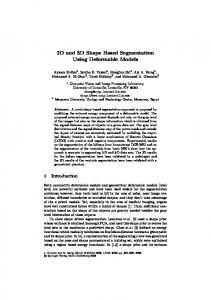
where L is the element’s characteristic length and c the sound speed in the material. To compute L the following procedure is adopted, see Figure 8: • Compute the twelve corner lengths s k , k = 1, …, 12 , to account for the element’s “stretching”. For example: s 1 = 12 .

39

(194)

• Build up the six mid-face points M f , f = 1, …, 6 . For example: 1 OM 1 = --- ( O1 + O2 + O3 + O4 ) 4

(195)

• Build up the three vectors a , b and c (which are only approximately perpendicular to each other): a = M3 M4

b = M5 M6

c = M1 M 2

(196)

• Compute the three “heights”, to take into account element’s “shearing”: (b × c) h a = a ⋅ ---------------b×c

(c × a) h b = b ⋅ ---------------c×a

(a × b) h c = c ⋅ ----------------- . a×b

(197)

• The characteristic length is the minimum of the computed lengths: L = min ( s 1, s 2, …, s 12, h a, h b, h c ) .

(198)

8 5

M2 c

M3

7

b M6 6

a 4

M5 x

1

O

M4 3

M1 2

Figure 8 - Computing the characteristic length for the 27-node element

An alternative calculation of L as the minimum intra-nodal distance between any couple of nodes can be activated by the option OPTI DTML.

40

4. Numerical examples Some numerical examples are presented illustrating the performance of the new elements introduced in the previous Sections.

4.1 Large-shear tests We start by some one-element large-shear tests inspired by the calculations performed in references [2-5] when discussing the treatment of large strains in 2D. The tests performed are summarized in Table 1. Name

Description

Steps

CPU (s)

SHEA11

Q41L

50000

5.44

SHEA12

Q42L

50000

5.10

SHEA13

C81L shear along x

50000

5.65

SHEA14

C82L shear along x

50000

5.37

SHEA15

C81L shear along y

50000

5.556

SHEA16

C82L shear along y

50000

5.46

SHEA17

C81L shear along z

50000

5.65

SHEA18

C82L shear along z

50000

6.15

Table 1 - Shear tests

SHEA11 This is a 2D plane strain calculation using the Q41L element, to be used as a reference for subsequent 3D calculations. The problem is shown in Figure 9. A square is subjected to a large shearing by blocking the base and by imposing horizontal displacements to the other nodes of the element as shown in the Figure. The material is assumed elastic.

y

x Figure 9 - The large shear problem in 2D.

41

The outcome of the calculation is the shear stress in the element which, according to the ZarembaJaumann-Noll formulation, has a periodic (sinusoidal) variation. In this case the maximum imposed horizontal displacement at the top of the element is 10 times the element length over a time span of 1 second. The imposed displacements are shown in Figure 10 and the resulting stresses are shown in Figure 11. The stresses have a sinusoidal shape, as expected. SHEA12 This is a repetition of test SHEA12 by using the Q42L (fully integrated) element instead of Q41L (reduced integrated). The results are practically identical as shown for example in Figure 12 for the shear stress. SHEA13 This test is 3D and uses the C81L under-integrated hexahedron element. The base of the element (in the x - y plane) is blocked in all directions. All other nodes are blocked in the y and z directions and are assigned suitable displacements along x , corresponding to those of the previous 2D cases. SHEA14 This test is similar to SHEA13 but uses the C82L fully-integrated element. SHEA05 This test is similar to SHEA13 but the shearing occurs along the y -direction. SHEA06 This test is similar to SHEA15 but uses the C82L fully-integrated element. SHEA07 This test is similar to SHEA13 but the shearing occurs along the z -direction. SHEA08 This test is similar to SHEA17 but uses the C82L fully-integrated element. Comparisons The results of all these 3D tests are all very similar and in very good agreement with the 2D reference. A comparison of the corresponding shear stresses is shown in Figure 13.

42

Figure 10 - Displacements in case SHEA11.

Figure 11 - Stresses in case SHEA11.

43

Figure 12 - Comparison of shear stresses in cases SHEA11 and SHEA12.

Figure 13 - Comparison of shear stresses in cases SHEA11 to SHEA18.

44

4.2 Large-rotation tests The next series of tests is used to check large rotations. An elastic beam of square cross section and length equal to ten times the cross-section side is subjected to an applied pressure along the whole length of the beam and is clamped at one extremity. This test is inspired from a similar test reported in reference [11]. The tests performed are summarized in Table 2. Name

Description

Steps

CPU (s)

POUT54

Q42L + CL22

5814

1.78

POU201

C81L + CL3Q

12034

12.57

POU202

C82L + CL3Q

11682

33.79

POU203

C81L + CL3Q rotated around x

11784

12.34

POU204

C81L + CL3Q rotated around y

12034

12.46

Table 2 - Pressurized beam tests

POUT54 This is a 2D plane strain calculation [11] using the Q42L linear quadrilateral and the CL22 boundary condition element to represent the applied pressure. This solution is then used as a reference for the subsequent 3D calculations. The beam undergoes very large displacements and rotations. Figure 14 shows the initial beam configuration and the deformed configuration at 3 ms, corresponding approximately to the maximum deflection. Figure 15 shows the displacements of the nodes at the free beam end. POU201 This is a 3D calculation using C81L and CL3Q (under-integrated) elements. POU202 This test is similar to POU201 but uses C82L and CL3Q (fully-integrated) elements. POU203 This test is similar to POU201 but the beam is rotated by 90° around the x -axis. POU204 This test is similar to POU201 but the beam is rotated by 90° around the y -axis.

45

Comparisons A comparison of the corresponding displacement of the mid-node at the free beam tip is shown in Figure 16 for all these tests. Two sets of curves are obtained: a set of slightly “stiffer” solutions is obtained by the fully-integrated elements, while a set of slightly “weaker” solutions is obtained by the reduced-integrated elements. The discrepancy is larger than in the case of parabolic elements (see Section 4.2 of reference [6]). In the case of reduced-integrated elements, some small mechanisms are observed.

Figure 14 - Deformations in case POUT54.

46

Figure 15 - Displacements in case POUT54.

Figure 16 - Comparison of displacements in cases POUT54 to POU204.

47

4.3 Elastic wave propagation tests The next series of tests is used to check elastic wave propagation. An elastic beam of square cross section and length equal to one hundred times the cross-section side is subjected to an initial velocity and is clamped at one extremity. The tests performed are summarized in Table 3. Name

Description

Steps

CPU (s)

BARE11

Q41L

800

0.59

BARE12

Q42L

800

0.69

BARE13

C81L

800

0.73

BARE14

C82L

800

1.05

Table 3 - Elastic wave propagation tests

BARE11 This is a 2D plane stress calculation using the Q41L linear quadrilateral. This solution is then used as a reference for the subsequent 3D calculations. The resulting stress at two points close to the bar mid-point are compared in Figure 17 against the analytical solution of the problem (a double step function). BARE12 This test is similar to BARE11 but uses the Q42L element. BARE03 This test is similar to BARE11 but uses the C81L element. BARE04 This test is similar to BARE11 but uses the C82L element. Comparison The results of these tests are all very similar and in very good agreement with the 2D reference. A comparison of the corresponding stress at the mid-point of the bar is shown in Figures 18 (using the average stress in the element to the left of the bar mid-point) and 19 (using the average stress in the element to the right of the bar mid-point).

48

Figure 17 - Stress in case BARE11 compared with the analytical solution.

Figure 18 - Stress in test cases BARE11 to BARE14 compared with the analytical solution.

49

Figure 19 - Stress in test cases BARE11 to BARE14 compared with the analytical solution.

4.4 Elasto-plastic bar impact test The next series of tests is used to check elasto-plasticity in large-strain deformation. The test is a classical elasto-plastic bar impact test, see e.g reference [12]. The tests performed are summarized in Table 4. Name

Description

Steps

CPU (s)

BARI23

Q41L, OPTI PART

2,760 macro

13.8

BARI24

C81L

(17,225 for 26 μs)

(11.8)

BARI25

C82L, 12 × 40

4,115

8.9

BARI26

Q42L, OPTI PART

2,802 macro

20.5

BARI30

Q42L

34,088

51.3

BARI31

Q41L

38,998

32.9

BARI32

Q42L, OPTI PART PLIN

2,802 macro

13.5

BARI33

Q41L, OPTI PART PLIN

2,760 macro

9.2

Table 4 - Elasto-plastic bar impact tests

50

BARI23 This is a 2D plane axisymmetric calculation using the Q41L linear quadrilaterals. The mesh (1/2 of the bar cross-section by symmetry) uses 12 × 120 linear elements. This solution is then used as a reference for the subsequent 3D calculations. The resulting radial and axial maximum displacements are shown in Figure 20 and are in excellent agreement with the solutions obtained in reference [6] with the parabolic elements. This calculation uses time step partitioning (OPTI PART) to decrease the CPU time. BARI24 This is a 3D calculation using the C81L linear hexahedron. The mesh (1/4 of the bar), shown in Figure 21, is relatively coarse and uses 12 × 40 elements. The calculation stops at about 26 μs because the element near the center of the impacting section becomes too squeezed and therefore the stability time step drops unacceptably. Displacements are compared in Figure 22 with the reference solution, showing excellent agreement as long as the 3D simulation is capable of advancing in time. The deformed mesh at calculation stop is shown in Figure 23. BARI25 This is a 3D calculation using the C82L linear hexahedron. The mesh is the same as in case BARI24. This calculation reaches without problems the final time of 80 μs. However, the solution exhibits severe locking (the deformation of the bar is largely underestimated). Displacements are compared in Figure 24 with the reference solution. The deformed mesh at calculation stop is shown in Figure 25. Due to the presence of severe locking, no further solutions with C82L are attempted. BARI26 This calculation is similar to BARI23 but uses the Q42L element instead of Q41L. Displacements are compared in Figure 26 with the reference solution, showing poor agreement. The 2D fully integrated solution exhibits some locking, although less pronounced than in the 3D fully integrated case. BARI30 This is a repetition of test BARI26 but without time step partitioning. Results are nearly identical to those of case BARI26 as shown in Figure 27, and the speed-up (in case BARI26) is about 2.5 times.

51

BARI31 This is a repetition of test BARI23 but without time step partitioning. Results are nearly identical to those of case BARI23 as shown in Figure 28, and the speed-up (in case BARI23) is about 2.4 times. BARI32 This is a repetition of test BARI26 but using the LINK COUP directive instead of LIAI and the OPTI PART PLIN option for time step partitioning. Results are nearly identical to those of case BARI26 as shown in Figure 29, and the further speed-up (with respect to BARI26) is about 33%. BARI33 This is a repetition of test BARI23 but using the LINK COUP directive instead of LIAI and the OPTI PART PLIN option for time step partitioning. Results are nearly identical to those of case BARI23 as shown in Figure 30, and the further speed-up (with respect to BARI23) is about 33%.

52

Figure 20 - Displacements in case BARI23.

Figure 21 - 3D mesh of case BARI24.

53

Figure 22 - Displacements in cases BARI23 and BARI24.

Deformed mesh

Three elements in the impact zone

Figure 23 - Mesh details of case BARI24 at calculation failure.

54

Figure 24 - Displacements in cases BARI23 and BARI25.

Figure 25 - Mesh details of case BARI25 at the final time.

55

Figure 26 - Displacements in cases BARI23 and BARI26.

Figure 27 - Displacements in cases BARI26 and BARI30.

56

Figure 28 - Displacements in cases BARI23 and BARI31.

Figure 29 - Displacements in cases BARI26 and BARI32.

57

Figure 30 - Displacements in cases BARI23 and BARI33.

58

5. References [1] “EUROPLEXUS User’s Manual”, on-line version: http://europlexus.jrc.ec.europa.eu. [2] J. P. HALLEUX, F. CASADEI: “Transient large strain analysis of plane and axisymmetric structures by means of biquadratic finite elements”. 2nd Int. Conf. on Numerical Methods for Nonlinear Problems, Barcelona, Apr. 9-13, 1984. [3] J. P. HALLEUX, F. CASADEI: “Transient large strain analysis of plane and axisymmetric structures by means of biquadratic finite elements”. Engineering Computations, Vol. 1, pp. 351-358, Dec. 1984. [4] F. CASADEI, J. DONEA, S. GIULIANI, J. P. HALLEUX, G. VERZELETTI: “Recenti sviluppi nei metodi computazionali e sperimentali per l’ analisi dinamica di strutture nel campo nonlineare”. XIII Convegno Nazionale dell’ Associazione Italiana per l’ Analisi delle Sollecitazioni, presso l’ I.S.M.E.S, Bergamo, 23-27 Settembre 1985. [5] J. P. HALLEUX, F. CASADEI: “Transient large strain finite element analysis of solids’. In ‘Computational Methods for Non-Linear Problems’, 2nd Volume in the Series: Recent Advances in Non-Linear Computational Mechanics, Eds. C. Taylor, D.R.J. Owen and E. Hinton, Pineridge Press, Swansea, 1987. [6] F. CASADEI: “Implementation of Parabolic Lagrange 2D and 3D Continuum Elements in EUROPLEXUS”. Technical Note Pubsy N. JRC66266, 2011. [7] F. CASADEI: “The LOOM System Raster Graphics Model”. Technical Note N. I.03.165, November 2003. [8] T.J.R. HUGHES, W.K. LIU: “Nonlinear finite element analysis of shells: Part I - three-dimensional shells”, Comp. Meths. Appl. Mech. Eng., 26, pp. 331-362, 1981. [9] T.J.R. HUGHES, W.K. LIU, I. LEVIT: “Nonlinear dynamic finite element analysis of shells”, in Nonlinear Finite Element Analysis in Structural Mechanics, Eds. W. Wunderlich et al., Springer, Berlin, 1981. [10] F. CASADEI: “A Nonlinear 3-D Shell Finite Element Implementation for Transient Problems”, Technical Note N. I.93.41, April 1993. [11] F. CASADEI: “Implementation of 3D Degenerated Shell Elements in PLEXIS-3C”, Technical Note N. I.93.88, July 1993. [12] F. CASADEI, J. DONEA, A. HUERTA: “Arbitrary Lagrangian-Eulerian Finite Elements in NonLinear Fast Transient Continuum Mechanics”, EUR 16327 EN, 1995.

59

bare11.dgibi

12 January 2015 2:26 pm

6. Appendix Sample input files This Section contains, in alphabetical file order, the listings of all input files related to the examples which were proposed in the previous Sections.

elim tol (bar1 et bar2); bar = (bar1 et bar2) coul vert; e1 = bar1 elem cont p3; e2 = bar2 elem cont p3; bartip = bar2 elem cont p2; mesh = bar et e1 et e2 et bartip; tass mesh; opti sauv form 'bare12.msh'; sauv form mesh; opti trac psc ftra 'bare12_mesh.ps'; trac qual mesh; fin;

bare12.epx BARE12 ECHO !CONV win CAST mesh CPLA LAGR GEOM Q42L COMP NGRO EPAI MATE VM23

bare11.dgibi *%siz†100 opti echo 1; opti dime 2 elem qua4; p1 = 0 0; p2 = 1 0; p3 = 0.5 0; tol = 0.001; dy = 0.01; n = 50; bar11 = (p1 d n p3) coul vert; bar21 = (p3 d n p2) coul vert; bar1 = (bar11 tran 1 (0 dy)) coul vert; bar2 = (bar21 tran 1 (0 dy)) coul vert; elim tol (bar1 et bar2); bar = (bar1 et bar2) coul vert; e1 = bar1 elem cont p3; e2 = bar2 elem cont p3; bartip = bar2 elem cont p2; mesh = bar et e1 et e2 et bartip; tass mesh; opti sauv form 'bare11.msh'; sauv form mesh; opti trac psc ftra 'bare11_mesh.ps'; trac qual mesh; fin;

LINK INIT ECRI

bare11.epx BARE11 ECHO !CONV win CAST mesh CPLA LAGR GEOM Q41L COMP NGRO EPAI MATE VM23

LINK INIT ECRI

bar TERM 1 'end' LECT bar TERM COND X GT 0.999 2.5E-8 LECT bar TERM RO 8000. YOUN 2.0E11 NU 0.0 ELAS 2.0E11 TRAC 1 2.0E11 1.E0 LECT bar TERM COUP BLOQ 1 LECT end TERM VITE 1 100.0 LECT bar DIFF end TERM DEPL VITE CONT ECRO TFREQ 0.1E-3 FICH ALIC TEMP FREQ 1 POIN LECT p3 p2 TERM ELEM LECT e1 e2 TERM FICH ALIC FREQ 1 PAS UTIL NOTE LOG 1 TINI 0. TEND 4.0E-4 PASF 5.0E-7

OPTI CALC SUIT Post-treatment ECHO RESU ALIC TEMP GARD PSCR SORT GRAP AXTE 1.0 'Time [s]' COUR 1 'dx_2' DEPL COMP 1 NOEU LECT COUR 2 'dx_3' DEPL COMP 1 NOEU LECT COUR 3 'sg_1' CONT COMP 1 ELEM LECT COUR 4 'sg_2' CONT COMP 1 ELEM LECT DCOU 5 'Analytical' 6 0.0 0.0 0.1E-3 0.0 0.1E-3 -4.E9 0.3E-3 -4.E9 0.3E-3 0.0 0.4E-3 0.0 TRAC 1 AXES 1.0 'DISPL. [M]' TRAC 2 AXES 1.0 'DISPL. [M]' TRAC 3 AXES 1.0 'CONTR. [PA]' TRAC 4 AXES 1.0 'CONTR. [PA]' TRAC 5 3 4 AXES 1.0 'CONTR. [PA]' YZER COLO ROUG NOIR NOIR DASH 2 0 0 LIST 1 AXES 1.0 'DISPL. [M]' LIST 2 AXES 1.0 'DISPL. [M]' LIST 3 AXES 1.0 'CONTR. [PA]' LIST 4 AXES 1.0 'CONTR. [PA]' FIN

p2 p3 e1 e2

TERM TERM TERM TERM

bar TERM 1 'end' LECT bar TERM COND X GT 0.999 2.5E-8 LECT bar TERM RO 8000. YOUN 2.0E11 NU 0.0 ELAS 2.0E11 TRAC 1 2.0E11 1.E0 LECT bar TERM COUP BLOQ 1 LECT end TERM VITE 1 100.0 LECT bar DIFF end TERM DEPL VITE CONT ECRO TFREQ 0.1E-3 FICH ALIC TEMP FREQ 1 POIN LECT p3 p2 TERM ELEM LECT e1 e2 TERM FICH ALIC FREQ 1 PAS UTIL NOTE LOG 1 TINI 0. TEND 4.0E-4 PASF 5.0E-7

OPTI CALC SUIT Post-treatment ECHO RESU ALIC TEMP GARD PSCR SORT GRAP AXTE 1.0 'Time [s]' COUR 1 'dx_2' DEPL COMP 1 NOEU LECT COUR 2 'dx_3' DEPL COMP 1 NOEU LECT COUR 3 'sg_1' CONT COMP 1 ELEM LECT COUR 4 'sg_2' CONT COMP 1 ELEM LECT DCOU 5 'Analytical' 6 0.0 0.0 0.1E-3 0.0 0.1E-3 -4.E9 0.3E-3 -4.E9 0.3E-3 0.0 0.4E-3 0.0 TRAC 1 AXES 1.0 'DISPL. [M]' TRAC 2 AXES 1.0 'DISPL. [M]' TRAC 3 AXES 1.0 'CONTR. [PA]' TRAC 4 AXES 1.0 'CONTR. [PA]' TRAC 5 3 4 AXES 1.0 'CONTR. [PA]' YZER COLO ROUG NOIR NOIR DASH 2 0 0 LIST 1 AXES 1.0 'DISPL. [M]' LIST 2 AXES 1.0 'DISPL. [M]' LIST 3 AXES 1.0 'CONTR. [PA]' LIST 4 AXES 1.0 'CONTR. [PA]' FIN

p2 p3 e1 e2

TERM TERM TERM TERM

bare13.dgibi *%siz†100 opti echo 1; opti dime 3 elem cub8; p1 = 0 0 0; p2 = 1 0 0; p3 = 0.5 0 0; tol = 0.001; dy = 0.01; dz = 0.01; n = 50; bas11 = (p1 d n p3) coul vert; bas21 = (p3 d n p2) coul vert; bas1 = (bas11 tran 1 (0 dy 0)) coul vert; bas2 = (bas21 tran 1 (0 dy 0)) coul vert; bar1 = bas1 volu tran 1 (0 0 dz); bar2 = bas2 volu tran 1 (0 0 dz); elim tol (bar1 et bar2); bar = (bar1 et bar2) coul vert; elim tol bar; mesh = bar; tass mesh; opti sauv form 'bare13.msh'; sauv form mesh; opti trac psc ftra 'bare13_mesh.ps'; trac cach qual (bar1 et bar2); fin;

bare13.epx bare12.dgibi *%siz†100 opti echo 1; opti dime 2 elem qua4; p1 = 0 0; p2 = 1 0; p3 = 0.5 0; tol = 0.001; dy = 0.01; n = 50; bar11 = (p1 d n p3) coul vert; bar21 = (p3 d n p2) coul vert; bar1 = (bar11 tran 1 (0 dy)) coul vert; bar2 = (bar21 tran 1 (0 dy)) coul vert;

BARE13 ECHO !CONV win CAST mesh TRID LAGR GEOM C81L bar TERM COMP GROU 2 'e1' LECT bar TERM COND XB GT 0.49 COND XB LT 0.50 'e2' LECT bar TERM COND XB LT 0.51 COND XB GT 0.50 NGRO 1 'end' LECT bar TERM COND X GT 0.999 MATE VM23 RO 8000. YOUN 2.0E11 NU 0.0 ELAS 2.0E11 TRAC 1 2.0E11 1.E0 LECT bar TERM LINK COUP BLOQ 1 LECT end TERM

Page 60

bare14.dgibi INIT VITE 1 100.0 LECT bar DIFF end TERM ECRI DEPL VITE CONT ECRO TFREQ 0.1E-3 FICH ALIC TEMP FREQ 1 POIN LECT p3 p2 TERM ELEM LECT e1 e2 TERM FICH ALIC FREQ 1 OPTI PAS UTIL NOTE LOG 1 CALC TINI 0. TEND 4.0E-4 PASF 5.0E-7 SUIT Post-treatment ECHO RESU ALIC TEMP GARD PSCR SORT GRAP AXTE 1.0 'Time [s]' COUR 1 'dx_2' DEPL COMP 1 NOEU LECT p2 COUR 2 'dx_3' DEPL COMP 1 NOEU LECT p3 COUR 3 'sg_1' CONT COMP 1 ELEM LECT e1 COUR 4 'sg_2' CONT COMP 1 ELEM LECT e2 DCOU 5 'Analytical' 6 0.0 0.0 0.1E-3 0.0 0.1E-3 -4.E9 0.3E-3 -4.E9 0.3E-3 0.0 0.4E-3 0.0 TRAC 1 AXES 1.0 'DISPL. [M]' TRAC 2 AXES 1.0 'DISPL. [M]' TRAC 3 AXES 1.0 'CONTR. [PA]' TRAC 4 AXES 1.0 'CONTR. [PA]' TRAC 5 3 4 AXES 1.0 'CONTR. [PA]' YZER COLO ROUG NOIR NOIR DASH 2 0 0 LIST 1 AXES 1.0 'DISPL. [M]' LIST 2 AXES 1.0 'DISPL. [M]' LIST 3 AXES 1.0 'CONTR. [PA]' LIST 4 AXES 1.0 'CONTR. [PA]' FIN

12 January 2015 2:26 pm TRAC 5 3 4 AXES COLO DASH LIST 1 AXES 1.0 LIST 2 AXES 1.0 LIST 3 AXES 1.0 LIST 4 AXES 1.0 FIN

1.0 'CONTR. [PA]' YZER ROUG NOIR NOIR 2 0 0 'DISPL. [M]' 'DISPL. [M]' 'CONTR. [PA]' 'CONTR. [PA]'

bare14c.epx TERM TERM TERM TERM

BARE14C ECHO RESU ALIC TEMP 'bare14.alt' GARD PSCR SORT GRAP AXTE 1.0 'Time [s]' COUR 43 'sg_1' CONT COMP 1 ELEM LECT e1 TERM COUR 44 'sg_2' CONT COMP 1 ELEM LECT e2 TERM DCOU 45 'Analytical' 6 0.0 0.0 0.1E-3 0.0 0.1E-3 -4.E9 0.3E-3 -4.E9 0.3E-3 0.0 0.4E-3 0.0 RCOU 13 'sg_1' FICH 'bare11.pun' RENA 'sg_1_11' RCOU 14 'sg_2' FICH 'bare11.pun' RENA 'sg_2_11' RCOU 23 'sg_1' FICH 'bare12.pun' RENA 'sg_1_12' RCOU 24 'sg_2' FICH 'bare12.pun' RENA 'sg_2_12' RCOU 33 'sg_1' FICH 'bare13.pun' RENA 'sg_1_13' RCOU 34 'sg_2' FICH 'bare13.pun' RENA 'sg_2_13' TRAC 13 23 33 43 45 AXES 1.0 'CONTR. [PA]' YZER COLO NOIR BLEU TURQ VERT ROUG TRAC 14 24 34 44 45 AXES 1.0 'CONTR. [PA]' YZER COLO NOIR BLEU TURQ VERT ROUG FIN

bare14.dgibi *%siz†100 opti echo 1; opti dime 3 elem cub8; p1 = 0 0 0; p2 = 1 0 0; p3 = 0.5 0 0; tol = 0.001; dy = 0.01; dz = 0.01; n = 50; bas11 = (p1 d n p3) coul vert; bas21 = (p3 d n p2) coul vert; bas1 = (bas11 tran 1 (0 dy 0)) coul vert; bas2 = (bas21 tran 1 (0 dy 0)) coul vert; bar1 = bas1 volu tran 1 (0 0 dz); bar2 = bas2 volu tran 1 (0 0 dz); elim tol (bar1 et bar2); bar = (bar1 et bar2) coul vert; elim tol bar; mesh = bar; tass mesh; opti sauv form 'bare14.msh'; sauv form mesh; opti trac psc ftra 'bare14_mesh.ps'; trac cach qual (bar1 et bar2); fin;

bare14.epx BARE14 ECHO !CONV win CAST mesh TRID LAGR GEOM C82L bar TERM COMP GROU 2 'e1' LECT bar TERM COND XB GT 0.49 COND XB LT 0.50 'e2' LECT bar TERM COND XB LT 0.51 COND XB GT 0.50 NGRO 1 'end' LECT bar TERM COND X GT 0.999 MATE VM23 RO 8000. YOUN 2.0E11 NU 0.0 ELAS 2.0E11 TRAC 1 2.0E11 1.E0 LECT bar TERM LINK COUP BLOQ 1 LECT end TERM INIT VITE 1 100.0 LECT bar DIFF end TERM ECRI DEPL VITE CONT ECRO TFREQ 0.1E-3 FICH ALIC TEMP FREQ 1 POIN LECT p3 p2 TERM ELEM LECT e1 e2 TERM FICH ALIC FREQ 1 OPTI PAS UTIL NOTE LOG 1 CALC TINI 0. TEND 4.0E-4 PASF 5.0E-7 SUIT Post-treatment ECHO RESU ALIC TEMP GARD PSCR SORT GRAP AXTE 1.0 'Time [s]' COUR 1 'dx_2' DEPL COMP 1 NOEU LECT p2 TERM COUR 2 'dx_3' DEPL COMP 1 NOEU LECT p3 TERM COUR 3 'sg_1' CONT COMP 1 ELEM LECT e1 TERM COUR 4 'sg_2' CONT COMP 1 ELEM LECT e2 TERM DCOU 5 'Analytical' 6 0.0 0.0 0.1E-3 0.0 0.1E-3 -4.E9 0.3E-3 -4.E9 0.3E-3 0.0 0.4E-3 0.0 TRAC 1 AXES 1.0 'DISPL. [M]' TRAC 2 AXES 1.0 'DISPL. [M]' TRAC 3 AXES 1.0 'CONTR. [PA]' TRAC 4 AXES 1.0 'CONTR. [PA]'

bari23.dgibi opti echo 1; opti titr 'BARI23'; opti trac psc ftra 'bari23_mesh.ps'; opti dime 2 elem qua4; p0=0 0; p1=3.2E-3 0; p2=0 32.4E-3; tol=0.01E-3; base=p0 d 12 p1; stru=base TRAN 120 p2; symax=stru poin droi p0 p2 tol; top=stru poin droi p2 (p1 PLUS p2) tol; elax=stru ELEM APPU LARG symax; elot=diff stru elax; str1=chan 'POI1' stru; bas1=chan 'POI1' base; viti=diff str1 bas1; mesh=stru et symax et viti; tass mesh; opti sauv form 'bari23.msh'; sauv form mesh; trac qual mesh; fin;

bari23.epx BARI23 ECHO !CONV WIN CAST mesh LAGR AXIS GEOM Q41L elax Q41L elot TERM COMP EPAI 1 LECT tous TERM MATE VM23 RO 8930. YOUN 1.17D11 NU 0.35D0 ELAS 4.D8 TRAC 2 4.D8 3.418803D-03 1.004D11 1000.003418803 LECT tous TERM LIAI BLOQ 2 LECT base TERM CONT SPLA NX 1 NY 0 LECT symax TERM INIT VITE 2 -227. LECT viti TERM ECRI DEPL VITE TFRE 10.E-6 POIN LECT p1 top TERM FICH ALIC TFRE 10.E-6 FICH ALIC TEMP TFRE 1.E-7 POIN LECT p1 top TERM OPTI PART NOTE CSTA 0.5 STEP IO LOG 1 CALC TINI 0. TEND 80.D-6 FIN

bari23a.epx BARI23A ECHO CONV WIN RESU ALIC 'bari23.ali' GARD PSCR SORT VISU NSTO 9 FIN

bari23b.epx Post-treatment (time curves ECHO RESU ALIC TEMP 'bari23.alt' COMP NGRO 2 'p0b' LECT tous 'p1b' LECT tous SORT GRAP AXTE 1.0 'Time [s]'

Page 61

from alice temps file) GARD PSCR TERM COND NEAR POIN 0.0 3.24E-2 TERM COND NEAR POIN 3.2E-3 3.24E-2

bari24.dgibi COUR COUR COUR TRAC LIST FIN

1 2 3 1 1

'dx_p1' 'dy_p0b' 'dy_p1b' 2 3 AXES 2 3 AXES

12 January 2015 2:26 pm DEPL COMP 1 DEPL COMP 2 DEPL COMP 2 1.0 'DISPL. 1.0 'DISPL.

POIN POIN POIN [M]' [M]'

LECT p1 TERM LECT p0b TERM LECT p1b TERM YZER YZER

bari24.dgibi

3 'dz_p1b' DEPL COMP 3 POIN LECT p1b TERM 4 'dz_p2b' DEPL COMP 3 POIN LECT p2b TERM 1 2 3 4 AXES 1.0 'DISPL. [M]' YZER 1 2 3 4 AXES 1.0 'DISPL. [M]' YZER 11 'dx_p1' FICH 'bari23b.pun' RENA 'dx_p1_23' 12 'dy_p0b' FICH 'bari23b.pun' RENA 'dy_p0b_23' 13 'dy_p1b' FICH 'bari23b.pun' RENA 'dy_p1b_23' 11 12 13 1 2 3 4 AXES 1.0 'DISPL. [M]' YZER ROUG ROUG ROUG NOIR NOIR NOIR NOIR

FIN

opti echo 1; opti titr 'BARI24'; opti trac psc ftra 'bari24_mesh.ps'; opti dime 3 elem cub8; p0=0 0 0; p0p=0 0 32.4E-3; p1=3.2E-3 0 0; p2=0 3.2E-3 0; p3=1.6E-3 0 0; p4=p1 tour 45 p0 p0p; p5=0 1.6E-3 0; x3 y3 z3 = coor p3; x4 y4 z4 = coor p4; x5 y5 z5 = coor p5; x6 = (x3 + x4 + x5) / 3.0; y6 = (y3 + y4 + y5) / 3.0; z6 = (z3 + z4 + z5) / 3.0; p6 = x6 y6 z6; tol=0.01E-3; n = 2; nz = 40; c1 = p0 d n p3; c2 = p3 d n p6; c3 = p6 d n p5; c4 = p5 d n p0; base1 = dall c1 c2 c3 c4 plan; c1 = p3 d n p1; c2 = p1 c n p0 p4; c3 = p4 d n p6; c4 = p6 d n p3; base2 = dall c1 c2 c3 c4 plan; c1 = p6 d n p4; c2 = p4 c n p0 p2; c3 = p2 d n p5; c4 = p5 d n p6; base3 = dall c1 c2 c3 c4 plan; base=base1 et base2 et base3; elim tol base; list (nbel base); list (nbno base); stru=base volu tran nz p0p; trac cach qual stru; * mesh=stru; tass mesh; opti sauv form 'bari24.msh'; sauv form mesh; fin;

bari24.epx BARI24 ECHO !CONV WIN CAST mesh LAGR TRID GEOM C81L stru TERM COMP NGRO 5 'blox' LECT tous TERM COND X LT 1.E-5 'bloy' LECT tous TERM COND Y LT 1.E-5 'nbas' LECT tous TERM COND Z LT 1.E-5 'top' LECT tous TERM COND Z GT 32.39E-3 'viti' LECT tous DIFF nbas TERM GROU 1 'ebas' LECT tous TERM COND ZB LT 5.E-4 COUL ROSE LECT stru TERM MATE VM23 RO 8930. YOUN 1.17D11 NU 0.35D0 ELAS 4.D8 TRAC 2 4.D8 3.418803D-03 1.004D11 1000.003418803 LECT stru TERM LIAI BLOQ 3 LECT nbas TERM BLOQ 1 LECT blox TERM BLOQ 2 LECT bloy TERM INIT VITE 3 -227. LECT viti TERM ECRI DEPL VITE TFRE 10.E-6 POIN LECT p1 p2 top TERM FICH ALIC TFRE 10.E-6 FICH ALIC TEMP TFRE 1.E-7 POIN LECT p1 top TERM OPTI PAS AUTO NOTE CSTA 0.5 STEP IO LOG 1 CALC TINI 0. TEND 80.D-6 FIN

bari24a.epx Post-treatment ECHO RESU ALIC 'bari24.ali' GARD PSCR SORT VISU NSTO 5 FIN

bari24b.epx Post-treatment (time curves ECHO RESU ALIC TEMP 'bari24.alt' COMP NGRO 3 'p0b' LECT tous 'p1b' LECT tous 'p2b' LECT tous SORT GRAP AXTE 1.0 'Time [s]' COUR 1 'dx_p1' DEPL COMP 1 COUR 2 'dz_p0b' DEPL COMP 3

COUR COUR TRAC LIST RCOU RCOU RCOU TRAC COLO

from alice temps file) GARD TERM TERM TERM

PSCR COND NEAR POIN 0.0 0.0 3.24E-2 COND NEAR POIN 3.2E-3 0.0 3.24E-2 COND NEAR POIN 0.0 3.2E-3 3.24E-2

POIN LECT p1 TERM POIN LECT p0b TERM

bari24f.epx BARI24F ECHO CONV WIN RESU ALIC 'bari24.ali' GARD PSCR SORT VISU NSTO 4 FIN

bari25.dgibi opti echo 1; opti titr 'BARI25'; opti trac psc ftra 'bari25_mesh.ps'; opti dime 3 elem cub8; p0=0 0 0; p0p=0 0 32.4E-3; p1=3.2E-3 0 0; p2=0 3.2E-3 0; p3=1.6E-3 0 0; p4=p1 tour 45 p0 p0p; p5=0 1.6E-3 0; x3 y3 z3 = coor p3; x4 y4 z4 = coor p4; x5 y5 z5 = coor p5; x6 = (x3 + x4 + x5) / 3.0; y6 = (y3 + y4 + y5) / 3.0; z6 = (z3 + z4 + z5) / 3.0; p6 = x6 y6 z6; tol=0.01E-3; n = 2; nz = 40; c1 = p0 d n p3; c2 = p3 d n p6; c3 = p6 d n p5; c4 = p5 d n p0; base1 = dall c1 c2 c3 c4 plan; c1 = p3 d n p1; c2 = p1 c n p0 p4; c3 = p4 d n p6; c4 = p6 d n p3; base2 = dall c1 c2 c3 c4 plan; c1 = p6 d n p4; c2 = p4 c n p0 p2; c3 = p2 d n p5; c4 = p5 d n p6; base3 = dall c1 c2 c3 c4 plan; base=base1 et base2 et base3; elim tol base; list (nbel base); list (nbno base); stru=base volu tran nz p0p; trac cach qual stru; * mesh=stru; tass mesh; opti sauv form 'bari25.msh'; sauv form mesh; fin;

bari25.epx BARI25 ECHO !CONV WIN CAST mesh LAGR TRID GEOM C82L stru TERM COMP NGRO 5 'blox' LECT tous TERM COND X LT 1.E-5 'bloy' LECT tous TERM COND Y LT 1.E-5 'nbas' LECT tous TERM COND Z LT 1.E-5 'top' LECT tous TERM COND Z GT 32.39E-3 'viti' LECT tous DIFF nbas TERM GROU 1 'ebas' LECT tous TERM COND ZB LT 5.E-4 COUL ROSE LECT stru TERM MATE VM23 RO 8930. YOUN 1.17D11 NU 0.35D0 ELAS 4.D8 TRAC 2 4.D8 3.418803D-03 1.004D11 1000.003418803 LECT stru TERM LIAI BLOQ 3 LECT nbas TERM BLOQ 1 LECT blox TERM BLOQ 2 LECT bloy TERM INIT VITE 3 -227. LECT viti TERM ECRI DEPL VITE TFRE 10.E-6 POIN LECT p1 p2 top TERM FICH ALIC TFRE 10.E-6 FICH ALIC TEMP TFRE 1.E-7 POIN LECT p1 top TERM OPTI PAS AUTO NOTE CSTA 0.5 STEP IO LOG 1 CALC TINI 0. TEND 80.D-6 FIN

bari25a.epx Post-treatment ECHO RESU ALIC 'bari25.ali' GARD PSCR SORT VISU NSTO 9

Page 62

bari25b.epx FIN

bari25b.epx Post-treatment (time curves from alice temps file) ECHO RESU ALIC TEMP 'bari25.alt' GARD PSCR COMP NGRO 3 'p0b' LECT tous TERM COND NEAR POIN 0.0 0.0 3.24E-2 'p1b' LECT tous TERM COND NEAR POIN 3.2E-3 0.0 3.24E-2 'p2b' LECT tous TERM COND NEAR POIN 0.0 3.2E-3 3.24E-2 SORT GRAP AXTE 1.0 'Time [s]' COUR 1 'dx_p1' DEPL COMP 1 POIN LECT p1 TERM COUR 2 'dz_p0b' DEPL COMP 3 POIN LECT p0b TERM COUR 3 'dz_p1b' DEPL COMP 3 POIN LECT p1b TERM COUR 4 'dz_p2b' DEPL COMP 3 POIN LECT p2b TERM TRAC 1 2 3 4 AXES 1.0 'DISPL. [M]' YZER LIST 1 2 3 4 AXES 1.0 'DISPL. [M]' YZER RCOU 11 'dx_p1' FICH 'bari23b.pun' RENA 'dx_p1_23' RCOU 12 'dy_p0b' FICH 'bari23b.pun' RENA 'dy_p0b_23' RCOU 13 'dy_p1b' FICH 'bari23b.pun' RENA 'dy_p1b_23' TRAC 11 12 13 1 2 3 4 AXES 1.0 'DISPL. [M]' YZER COLO ROUG ROUG ROUG NOIR NOIR NOIR NOIR FIN

bari26.dgibi opti echo 1; opti titr 'BARI26'; opti trac psc ftra 'bari26_mesh.ps'; opti dime 2 elem qua4; p0=0 0; p1=3.2E-3 0; p2=0 32.4E-3; tol=0.01E-3; base=p0 d 12 p1; stru=base TRAN 120 p2; symax=stru poin droi p0 p2 tol; top=stru poin droi p2 (p1 PLUS p2) tol; elax=stru ELEM APPU LARG symax; elot=diff stru elax; str1=chan 'POI1' stru; bas1=chan 'POI1' base; viti=diff str1 bas1; mesh=stru et symax et viti; tass mesh; opti sauv form 'bari26.msh'; sauv form mesh; trac qual mesh; fin;

bari26.epx BARI26 ECHO !CONV WIN CAST mesh LAGR AXIS GEOM Q42L elax Q42L elot TERM COMP EPAI 1 LECT tous TERM MATE VM23 RO 8930. YOUN 1.17D11 NU 0.35D0 ELAS 4.D8 TRAC 2 4.D8 3.418803D-03 1.004D11 1000.003418803 LECT tous TERM LIAI BLOQ 2 LECT base TERM CONT SPLA NX 1 NY 0 LECT symax TERM INIT VITE 2 -227. LECT viti TERM ECRI DEPL VITE TFRE 10.E-6 POIN LECT p1 top TERM FICH ALIC TFRE 10.E-6 FICH ALIC TEMP TFRE 1.E-7 POIN LECT p1 top TERM OPTI PART NOTE CSTA 0.5 STEP IO LOG 1 CALC TINI 0. TEND 80.D-6 FIN

bari26b.epx Post-treatment (time curves from alice temps file) ECHO RESU ALIC TEMP 'bari26.alt' GARD PSCR COMP NGRO 2 'p0b' LECT tous TERM COND NEAR POIN 0.0 3.24E-2 'p1b' LECT tous TERM COND NEAR POIN 3.2E-3 3.24E-2 SORT GRAP AXTE 1.0 'Time [s]' COUR 1 'dx_p1' DEPL COMP 1 POIN LECT p1 TERM COUR 2 'dy_p0b' DEPL COMP 2 POIN LECT p0b TERM COUR 3 'dy_p1b' DEPL COMP 2 POIN LECT p1b TERM TRAC 1 2 3 AXES 1.0 'DISPL. [M]' YZER LIST 1 2 3 AXES 1.0 'DISPL. [M]' YZER RCOU 11 'dx_p1' FICH 'bari23b.pun' RENA 'dx_p1_23' RCOU 12 'dy_p0b' FICH 'bari23b.pun' RENA 'dy_p0b_23' RCOU 13 'dy_p1b' FICH 'bari23b.pun' RENA 'dy_p1b_23' TRAC 11 12 13 1 2 3 AXES 1.0 'DISPL. [M]' YZER COLO ROUG ROUG ROUG NOIR NOIR NOIR FIN

bari30.dgibi opti echo opti titr opti trac opti dime p0=0 0; p1=3.2E-3

1; 'BARI30'; psc ftra 'bari30_mesh.ps'; 2 elem qua4; 0;

12 January 2015 2:26 pm p2=0 32.4E-3; tol=0.01E-3; base=p0 d 12 p1; stru=base TRAN 120 p2; symax=stru poin droi p0 p2 tol; top=stru poin droi p2 (p1 PLUS p2) tol; elax=stru ELEM APPU LARG symax; elot=diff stru elax; str1=chan 'POI1' stru; bas1=chan 'POI1' base; viti=diff str1 bas1; mesh=stru et symax et viti; tass mesh; opti sauv form 'bari30.msh'; sauv form mesh; trac qual mesh; fin;

bari30.epx BARI30 ECHO !CONV WIN CAST mesh LAGR AXIS GEOM Q42L elax Q42L elot TERM COMP EPAI 1 LECT tous TERM MATE VM23 RO 8930. YOUN 1.17D11 NU 0.35D0 ELAS 4.D8 TRAC 2 4.D8 3.418803D-03 1.004D11 1000.003418803 LECT tous TERM LIAI BLOQ 2 LECT base TERM CONT SPLA NX 1 NY 0 LECT symax TERM INIT VITE 2 -227. LECT viti TERM ECRI DEPL VITE TFRE 10.E-6 POIN LECT p1 top TERM FICH ALIC TFRE 10.E-6 FICH ALIC TEMP TFRE 1.E-7 POIN LECT p1 top TERM OPTI PAS AUTO NOTE CSTA 0.5 STEP IO LOG 1 CALC TINI 0. TEND 80.D-6 FIN

bari30b.epx Post-treatment (time curves from alice temps file) ECHO RESU ALIC TEMP 'bari30.alt' GARD PSCR COMP NGRO 2 'p0b' LECT tous TERM COND NEAR POIN 0.0 3.24E-2 'p1b' LECT tous TERM COND NEAR POIN 3.2E-3 3.24E-2 SORT GRAP AXTE 1.0 'Time [s]' COUR 1 'dx_p1' DEPL COMP 1 POIN LECT p1 TERM COUR 2 'dy_p0b' DEPL COMP 2 POIN LECT p0b TERM COUR 3 'dy_p1b' DEPL COMP 2 POIN LECT p1b TERM TRAC 1 2 3 AXES 1.0 'DISPL. [M]' YZER LIST 1 2 3 AXES 1.0 'DISPL. [M]' YZER RCOU 11 'dx_p1' FICH 'bari26b.pun' RENA 'dx_p1_26' RCOU 12 'dy_p0b' FICH 'bari26b.pun' RENA 'dy_p0b_26' RCOU 13 'dy_p1b' FICH 'bari26b.pun' RENA 'dy_p1b_26' TRAC 11 12 13 1 2 3 AXES 1.0 'DISPL. [M]' YZER COLO ROUG ROUG ROUG NOIR NOIR NOIR FIN

bari31.dgibi opti echo 1; opti titr 'BARI31'; opti trac psc ftra 'bari31_mesh.ps'; opti dime 2 elem qua4; p0=0 0; p1=3.2E-3 0; p2=0 32.4E-3; tol=0.01E-3; base=p0 d 12 p1; stru=base TRAN 120 p2; symax=stru poin droi p0 p2 tol; top=stru poin droi p2 (p1 PLUS p2) tol; elax=stru ELEM APPU LARG symax; elot=diff stru elax; str1=chan 'POI1' stru; bas1=chan 'POI1' base; viti=diff str1 bas1; mesh=stru et symax et viti; tass mesh; opti sauv form 'bari31.msh'; sauv form mesh; trac qual mesh; fin;

bari31.epx BARI31 ECHO !CONV WIN CAST mesh LAGR AXIS GEOM Q41L elax Q41L elot TERM COMP EPAI 1 LECT tous TERM MATE VM23 RO 8930. YOUN 1.17D11 NU 0.35D0 ELAS 4.D8 TRAC 2 4.D8 3.418803D-03 1.004D11 1000.003418803 LECT tous TERM LIAI BLOQ 2 LECT base TERM CONT SPLA NX 1 NY 0 LECT symax TERM INIT VITE 2 -227. LECT viti TERM ECRI DEPL VITE TFRE 10.E-6 POIN LECT p1 top TERM FICH ALIC TFRE 10.E-6 FICH ALIC TEMP TFRE 1.E-7

Page 63

bari31a.epx POIN LECT p1 top TERM OPTI PAS AUTO NOTE CSTA 0.5 STEP IO LOG 1 CALC TINI 0. TEND 80.D-6 FIN

12 January 2015 2:26 pm FIN

bari33.dgibi bari31a.epx BARI31A ECHO CONV WIN RESU ALIC 'bari31.ali' GARD PSCR SORT VISU NSTO 9 FIN

bari31b.epx Post-treatment (time curves from alice temps file) ECHO RESU ALIC TEMP 'bari31.alt' GARD PSCR COMP NGRO 2 'p0b' LECT tous TERM COND NEAR POIN 0.0 3.24E-2 'p1b' LECT tous TERM COND NEAR POIN 3.2E-3 3.24E-2 SORT GRAP AXTE 1.0 'Time [s]' COUR 1 'dx_p1' DEPL COMP 1 POIN LECT p1 TERM COUR 2 'dy_p0b' DEPL COMP 2 POIN LECT p0b TERM COUR 3 'dy_p1b' DEPL COMP 2 POIN LECT p1b TERM TRAC 1 2 3 AXES 1.0 'DISPL. [M]' YZER LIST 1 2 3 AXES 1.0 'DISPL. [M]' YZER RCOU 11 'dx_p1' FICH 'bari23b.pun' RENA 'dx_p1_23' RCOU 12 'dy_p0b' FICH 'bari23b.pun' RENA 'dy_p0b_23' RCOU 13 'dy_p1b' FICH 'bari23b.pun' RENA 'dy_p1b_23' TRAC 11 12 13 1 2 3 AXES 1.0 'DISPL. [M]' YZER COLO ROUG ROUG ROUG NOIR NOIR NOIR FIN

bari32.dgibi opti echo 1; opti titr 'BARI32'; opti trac psc ftra 'bari32_mesh.ps'; opti dime 2 elem qua4; p0=0 0; p1=3.2E-3 0; p2=0 32.4E-3; tol=0.01E-3; base=p0 d 12 p1; stru=base TRAN 120 p2; symax=stru poin droi p0 p2 tol; top=stru poin droi p2 (p1 PLUS p2) tol; elax=stru ELEM APPU LARG symax; elot=diff stru elax; str1=chan 'POI1' stru; bas1=chan 'POI1' base; viti=diff str1 bas1; mesh=stru et symax et viti; tass mesh; opti sauv form 'bari32.msh'; sauv form mesh; trac qual mesh; fin;

bari32.epx BARI32 ECHO !CONV WIN CAST mesh LAGR AXIS GEOM Q42L elax Q42L elot TERM COMP EPAI 1 LECT tous TERM MATE VM23 RO 8930. YOUN 1.17D11 NU 0.35D0 ELAS 4.D8 TRAC 2 4.D8 3.418803D-03 1.004D11 1000.003418803 LECT tous TERM LINK COUP BLOQ 2 LECT base TERM CONT SPLA NX 1 NY 0 LECT symax TERM INIT VITE 2 -227. LECT viti TERM ECRI DEPL VITE TFRE 10.E-6 POIN LECT p1 top TERM FICH ALIC TFRE 10.E-6 FICH ALIC TEMP TFRE 1.E-7 POIN LECT p1 top TERM OPTI PART PLIN NOTE CSTA 0.5 STEP IO LOG 1 CALC TINI 0. TEND 80.D-6 FIN

opti echo 1; opti titr 'BARI33'; opti trac psc ftra 'bari33_mesh.ps'; opti dime 2 elem qua4; p0=0 0; p1=3.2E-3 0; p2=0 32.4E-3; tol=0.01E-3; base=p0 d 12 p1; stru=base TRAN 120 p2; symax=stru poin droi p0 p2 tol; top=stru poin droi p2 (p1 PLUS p2) tol; elax=stru ELEM APPU LARG symax; elot=diff stru elax; str1=chan 'POI1' stru; bas1=chan 'POI1' base; viti=diff str1 bas1; mesh=stru et symax et viti; tass mesh; opti sauv form 'bari33.msh'; sauv form mesh; trac qual mesh; fin;

bari33.epx BARI33 ECHO !CONV WIN CAST mesh LAGR AXIS GEOM Q41L elax Q41L elot TERM COMP EPAI 1 LECT tous TERM MATE VM23 RO 8930. YOUN 1.17D11 NU 0.35D0 ELAS 4.D8 TRAC 2 4.D8 3.418803D-03 1.004D11 1000.003418803 LECT tous TERM LINK COUP BLOQ 2 LECT base TERM CONT SPLA NX 1 NY 0 LECT symax TERM INIT VITE 2 -227. LECT viti TERM ECRI DEPL VITE TFRE 10.E-6 POIN LECT p1 top TERM FICH ALIC TFRE 10.E-6 FICH ALIC TEMP TFRE 1.E-7 POIN LECT p1 top TERM OPTI PART PLIN NOTE CSTA 0.5 STEP IO LOG 1 CALC TINI 0. TEND 80.D-6 FIN

bari33a.epx BARI33A ECHO CONV WIN RESU ALIC 'bari33.ali' GARD PSCR SORT VISU NSTO 9 FIN

bari33b.epx Post-treatment (time curves from alice temps file) ECHO RESU ALIC TEMP 'bari33.alt' GARD PSCR COMP NGRO 2 'p0b' LECT tous TERM COND NEAR POIN 0.0 3.24E-2 'p1b' LECT tous TERM COND NEAR POIN 3.2E-3 3.24E-2 SORT GRAP AXTE 1.0 'Time [s]' COUR 1 'dx_p1' DEPL COMP 1 POIN LECT p1 TERM COUR 2 'dy_p0b' DEPL COMP 2 POIN LECT p0b TERM COUR 3 'dy_p1b' DEPL COMP 2 POIN LECT p1b TERM TRAC 1 2 3 AXES 1.0 'DISPL. [M]' YZER LIST 1 2 3 AXES 1.0 'DISPL. [M]' YZER RCOU 11 'dx_p1' FICH 'bari23b.pun' RENA 'dx_p1_23' RCOU 12 'dy_p0b' FICH 'bari23b.pun' RENA 'dy_p0b_23' RCOU 13 'dy_p1b' FICH 'bari23b.pun' RENA 'dy_p1b_23' TRAC 11 12 13 1 2 3 AXES 1.0 'DISPL. [M]' YZER COLO ROUG ROUG ROUG NOIR NOIR NOIR FIN

pou201.dgibi bari32b.epx Post-treatment (time curves from alice temps file) ECHO RESU ALIC TEMP 'bari32.alt' GARD PSCR COMP NGRO 2 'p0b' LECT tous TERM COND NEAR POIN 0.0 3.24E-2 'p1b' LECT tous TERM COND NEAR POIN 3.2E-3 3.24E-2 SORT GRAP AXTE 1.0 'Time [s]' COUR 1 'dx_p1' DEPL COMP 1 POIN LECT p1 TERM COUR 2 'dy_p0b' DEPL COMP 2 POIN LECT p0b TERM COUR 3 'dy_p1b' DEPL COMP 2 POIN LECT p1b TERM TRAC 1 2 3 AXES 1.0 'DISPL. [M]' YZER LIST 1 2 3 AXES 1.0 'DISPL. [M]' YZER RCOU 11 'dx_p1' FICH 'bari26b.pun' RENA 'dx_p1_26' RCOU 12 'dy_p0b' FICH 'bari26b.pun' RENA 'dy_p0b_26' RCOU 13 'dy_p1b' FICH 'bari26b.pun' RENA 'dy_p1b_26' TRAC 11 12 13 1 2 3 AXES 1.0 'DISPL. [M]' YZER COLO ROUG ROUG ROUG NOIR NOIR NOIR

opti titr 'pou201'; opti echo 1; opti dime 3 elem cub8; opti trac psc ftra 'pou201_mesh.ps'; p1=0 0 0;p2=10 0 0; p3=10 1 0;p4=0 1 0; p04 = 0 0.5 0.00; p14 = 0 0.5 0.25; p24 = 0 0.5 0.50; p34 = 0 0.5 0.75; p44 = 0 0.5 1.00; tol=0.001; * * define structural mesh * c1=p1 d 40 p2; c2=p2 d 4 p3; c3=p3 d 40 p4; c4=p4 d 4 p1; base=daller c1 c2 c3 c4 plan; pout=volu base tran 4 (0 0 1);

Page 64

pou201.epx * presslow = base; baseup = base plus (0 0 1); baseup = orie baseup poin (5 0.5 0); * pressup = baseup; elim tol (pout et pressup); elim tol (pout et p04 et p14 et p24 et p34 et p44); * pression=presslow et pressup; * * define total mesh object and eliminate double points * mesh = pout et pression; elim tol mesh; tass mesh; * * store the results * opti sauv form 'pou201.msh'; sauv form mesh; trac cach qual pout; trac cach qual (base et baseup); fin;

pou201.epx POU201 ECHO !CONV WIN CAST mesh LAGR TRID GEOM C81L pout CL3Q pression TERM COMP NGRO 1 'bloxz' LECT tous TERM COND X GT 9.99 MATE VM23 RO 1.030E-6 YOUN 1.2E4 NU 0.2 ELAS 1.32E4 TRAC 1 1.32E4 1.1 LECT pout TERM IMPE PIMP RO 0 PREF 0 PRES -1.425 TABP 2 0.0 1.0 1.0 1.0 LECT pressup TERM IMPE PIMP RO 0 PREF 0 PRES 1.425 TABP 2 0.0 1.0 1.0 1.0 LECT presslow TERM LINK COUP BLOQ 2 LECT tous TERM BLOQ 13 LECT bloxz TERM ECRI DEPL VITE CONT TFRE 3.D-3 FICH ALIC TFRE 1.E-3 FICH ALIC TEMP TFRE 1.E-5 POIN LECT p04 p14 p24 p34 p44 TERM OPTI PAS AUTO NOTE CSTA 0.5 STEP IO LOG 1 CALC TINI 0.0 TEND 6.E-3 SUIT Post-treatment (time curves from alice temps file) ECHO RESU ALIC TEMP GARD PSCR SORT GRAP AXTE 1.0 'Time [s]' COUR 1 'dz_p04' DEPL COMP 3 NOEU LECT p04 TERM COUR 2 'dz_p14' DEPL COMP 3 NOEU LECT p14 TERM COUR 3 'dz_p24' DEPL COMP 3 NOEU LECT p24 TERM COUR 4 'dz_p34' DEPL COMP 3 NOEU LECT p34 TERM COUR 5 'dz_p44' DEPL COMP 3 NOEU LECT p44 TERM TRAC 1 2 3 4 5 AXES 1.0 'DISPL. [M]' YZER LIST 1 2 3 4 5 AXES 1.0 'DISPL. [M]' FIN

pou201b.epx POU201B ECHO CONV WIN RESU ALIC 'pou201.ali' GARD PSCR SORT VISU NSTO 4 FIN

pou202.dgibi opti titr 'pou202'; opti echo 1; opti dime 3 elem cub8; opti trac psc ftra 'pou202_mesh.ps'; p1=0 0 0;p2=10 0 0; p3=10 1 0;p4=0 1 0; p04 = 0 0.5 0.00; p14 = 0 0.5 0.25; p24 = 0 0.5 0.50; p34 = 0 0.5 0.75; p44 = 0 0.5 1.00; tol=0.001; * * define structural mesh * c1=p1 d 40 p2; c2=p2 d 4 p3; c3=p3 d 40 p4; c4=p4 d 4 p1; base=daller c1 c2 c3 c4 plan; pout=volu base tran 4 (0 0 1); * presslow = base; baseup = base plus (0 0 1); baseup = orie baseup poin (5 0.5 0); * pressup = baseup; elim tol (pout et pressup); elim tol (pout et p04 et p14 et p24 et p34 et p44); * pression=presslow et pressup; * * define total mesh object and eliminate double points

12 January 2015 2:26 pm * mesh = pout et pression; elim tol mesh; tass mesh; * * store the results * opti sauv form 'pou202.msh'; sauv form mesh; trac cach qual pout; trac cach qual (base et baseup); fin;

pou202.epx POU202 ECHO !CONV WIN CAST mesh LAGR TRID GEOM C82L pout CL3Q pression TERM COMP NGRO 1 'bloxz' LECT tous TERM COND X GT 9.99 MATE VM23 RO 1.030E-6 YOUN 1.2E4 NU 0.2 ELAS 1.32E4 TRAC 1 1.32E4 1.1 LECT pout TERM IMPE PIMP RO 0 PREF 0 PRES -1.425 TABP 2 0.0 1.0 1.0 1.0 LECT pressup TERM IMPE PIMP RO 0 PREF 0 PRES 1.425 TABP 2 0.0 1.0 1.0 1.0 LECT presslow TERM LINK COUP BLOQ 2 LECT tous TERM BLOQ 13 LECT bloxz TERM ECRI DEPL VITE CONT TFRE 3.D-3 FICH ALIC TFRE 1.E-3 FICH ALIC TEMP TFRE 1.E-5 POIN LECT p04 p14 p24 p34 p44 TERM OPTI PAS AUTO NOTE CSTA 0.5 STEP IO LOG 1 CALC TINI 0.0 TEND 6.E-3 SUIT Post-treatment (time curves from alice temps file) ECHO RESU ALIC TEMP GARD PSCR SORT GRAP AXTE 1.0 'Time [s]' COUR 1 'dz_p04' DEPL COMP 3 NOEU LECT p04 TERM COUR 2 'dz_p14' DEPL COMP 3 NOEU LECT p14 TERM COUR 3 'dz_p24' DEPL COMP 3 NOEU LECT p24 TERM COUR 4 'dz_p34' DEPL COMP 3 NOEU LECT p34 TERM COUR 5 'dz_p44' DEPL COMP 3 NOEU LECT p44 TERM TRAC 1 2 3 4 5 AXES 1.0 'DISPL. [M]' YZER LIST 1 2 3 4 5 AXES 1.0 'DISPL. [M]' FIN

pou202b.epx POU202B ECHO CONV WIN RESU ALIC 'pou202.ali' GARD PSCR SORT VISU NSTO 4 FIN

pou203.dgibi opti titr 'pou203'; opti echo 1; opti dime 3 elem cub8; opti trac psc ftra 'pou203_mesh.ps'; p1=0 0 0;p2=10 0 0; p3=10 1 0;p4=0 1 0; p04 = 0 0.5 0.00; p14 = 0 0.5 0.25; p24 = 0 0.5 0.50; p34 = 0 0.5 0.75; p44 = 0 0.5 1.00; tol=0.001; * * define structural mesh * c1=p1 d 40 p2; c2=p2 d 4 p3; c3=p3 d 40 p4; c4=p4 d 4 p1; base=daller c1 c2 c3 c4 plan; pout=volu base tran 4 (0 0 1); * presslow = base; baseup = base plus (0 0 1); baseup = orie baseup poin (5 0.5 0); * pressup = baseup; elim tol (pout et pressup); elim tol (pout et p04 et p14 et p24 et p34 et p44); * pression=presslow et pressup; * * define total mesh object and eliminate double points * mesh = pout et pression; depl mesh tour 90 p2 p1; elim tol mesh; tass mesh; * * store the results * opti sauv form 'pou203.msh'; sauv form mesh; trac cach qual pout; trac cach qual (base et baseup);

Page 65

pou203.epx fin;

pou203.epx POU203 ECHO !CONV WIN CAST mesh LAGR TRID GEOM C81L pout CL3Q pression TERM COMP NGRO 1 'bloxy' LECT tous TERM COND X GT 9.99 MATE VM23 RO 1.030E-6 YOUN 1.2E4 NU 0.2 ELAS 1.32E4 TRAC 1 1.32E4 1.1 LECT pout TERM IMPE PIMP RO 0 PREF 0 PRES -1.425 TABP 2 0.0 1.0 1.0 1.0 LECT pressup TERM IMPE PIMP RO 0 PREF 0 PRES 1.425 TABP 2 0.0 1.0 1.0 1.0 LECT presslow TERM LINK COUP BLOQ 3 LECT tous TERM BLOQ 12 LECT bloxy TERM ECRI DEPL VITE CONT TFRE 3.D-3 FICH ALIC TFRE 1.E-3 FICH ALIC TEMP TFRE 1.E-5 POIN LECT p04 p14 p24 p34 p44 TERM OPTI PAS AUTO NOTE CSTA 0.5 STEP IO LOG 1 CALC TINI 0.0 TEND 6.E-3 SUIT Post-treatment (time curves from alice temps file) ECHO RESU ALIC TEMP GARD PSCR SORT GRAP AXTE 1.0 'Time [s]' COUR 1 'dy_p04' DEPL COMP 2 NOEU LECT p04 TERM COUR 2 'dy_p14' DEPL COMP 2 NOEU LECT p14 TERM COUR 3 'dy_p24' DEPL COMP 2 NOEU LECT p24 TERM COUR 4 'dy_p34' DEPL COMP 2 NOEU LECT p34 TERM COUR 5 'dy_p44' DEPL COMP 2 NOEU LECT p44 TERM TRAC 1 2 3 4 5 AXES 1.0 'DISPL. [M]' YZER LIST 1 2 3 4 5 AXES 1.0 'DISPL. [M]' FIN

12 January 2015 2:26 pm GEOM C81L pout CL3Q pression TERM COMP NGRO 1 'bloxz' LECT tous TERM COND Z LT -9.99 MATE VM23 RO 1.030E-6 YOUN 1.2E4 NU 0.2 ELAS 1.32E4 TRAC 1 1.32E4 1.1 LECT pout TERM IMPE PIMP RO 0 PREF 0 PRES -1.425 TABP 2 0.0 1.0 1.0 1.0 LECT pressup TERM IMPE PIMP RO 0 PREF 0 PRES 1.425 TABP 2 0.0 1.0 1.0 1.0 LECT presslow TERM LINK COUP BLOQ 2 LECT tous TERM BLOQ 13 LECT bloxz TERM ECRI DEPL VITE CONT TFRE 3.D-3 FICH ALIC TFRE 1.E-3 FICH ALIC TEMP TFRE 1.E-5 POIN LECT p04 p14 p24 p34 p44 TERM OPTI PAS AUTO NOTE CSTA 0.5 STEP IO LOG 1 CALC TINI 0.0 TEND 6.E-3 SUIT Post-treatment (time curves from alice temps file) ECHO RESU ALIC TEMP GARD PSCR SORT GRAP AXTE 1.0 'Time [s]' COUR 1 'dx_p04' DEPL COMP 1 NOEU LECT p04 TERM COUR 2 'dx_p14' DEPL COMP 1 NOEU LECT p14 TERM COUR 3 'dx_p24' DEPL COMP 1 NOEU LECT p24 TERM COUR 4 'dx_p34' DEPL COMP 1 NOEU LECT p34 TERM COUR 5 'dx_p44' DEPL COMP 1 NOEU LECT p44 TERM TRAC 1 2 3 4 5 AXES 1.0 'DISPL. [M]' YZER LIST 1 2 3 4 5 AXES 1.0 'DISPL. [M]' FIN

pou204b.epx POU204B ECHO CONV WIN RESU ALIC 'pou204.ali' GARD PSCR SORT VISU NSTO 4 FIN

pou203b.epx

pou204c.epx

POU203B ECHO CONV WIN RESU ALIC 'pou203.ali' GARD PSCR SORT VISU NSTO 4 FIN

POU204C ECHO RESU ALIC TEMP 'pou204.alt' GARD PSCR SORT GRAP AXTE 1.0 'Time [s]' COUR 43 'dx_p24' DEPL COMP 1 NOEU LECT p24 TERM RCOU 13 'dz_p24' FICH 'pou201.pun' RENA 'dz_p24_201' RCOU 23 'dz_p24' FICH 'pou202.pun' RENA 'dz_p24_202' RCOU 33 'dy_p24' FICH 'pou203.pun' RENA 'dy_p24_203' RCOU 44 'dy_p24' FICH 'pout54.pun' RENA 'dy_p24_54' TRAC 13 23 33 43 44 AXES 1.0 'DISPL. [M]' YZER COLO NOIR TURQ VERT ROUG ROSE FIN

pou204.dgibi opti titr 'pou204'; opti echo 1; opti dime 3 elem cub8; opti trac psc ftra 'pou204_mesh.ps'; p1=0 0 0;p2=10 0 0; p3=10 1 0;p4=0 1 0; p04 = 0 0.5 0.00; p14 = 0 0.5 0.25; p24 = 0 0.5 0.50; p34 = 0 0.5 0.75; p44 = 0 0.5 1.00; tol=0.001; * * define structural mesh * c1=p1 d 40 p2; c2=p2 d 4 p3; c3=p3 d 40 p4; c4=p4 d 4 p1; base=daller c1 c2 c3 c4 plan; pout=volu base tran 4 (0 0 1); * presslow = base; baseup = base plus (0 0 1); baseup = orie baseup poin (5 0.5 0); * pressup = baseup; elim tol (pout et pressup); elim tol (pout et p04 et p14 et p24 et p34 et p44); * pression=presslow et pressup; * * define total mesh object and eliminate double points * mesh = pout et pression; depl mesh tour 90 p1 p4; elim tol mesh; tass mesh; * * store the results * opti sauv form 'pou204.msh'; sauv form mesh; trac cach qual pout; trac cach qual (base et baseup); fin;

pou204.epx

pout54.dgibi opti titr 'pout54'; opti echo 1; opti dime 2 elem qua4; opti trac psc ftra 'pout54_mesh.ps'; p1=0 0;p2=10 0; p3=10 1;p4=0 1; p14 = 0 0.25; p24 = 0 0.50; p34 = 0 0.75; tol=0.001; * * define structural mesh * c1=p1 d 40 p2; c2=p2 d 4 p3; c3=p3 d 40 p4; c4=p4 d 4 p1; pout=daller c1 c2 c3 c4 plan; elim tol (pout et p14 et p24 et p34); * * define nodes subjected to blockages or TPLOT * bloc=pout poin droi p2 p3 tol; tpln=pout poin droi p1 p4 tol; * * define applied pressure elements * opti elem seg2; presslow=p1 d 40 p2; pressup=p3 d 40 p4; pression=presslow et pressup; * * define total mesh object and eliminate double points * mesh=pout et pression et bloc et tpln; elim tol mesh; tass mesh; * * store the results * opti sauv form 'pout54.msh'; sauv form mesh; trac qual mesh; fin;

POU204 ECHO !CONV WIN CAST mesh LAGR TRID

Page 66

pout54.epx

pout54.epx POUT54 - 2D Q42L+CL22 DOUBLE LAYER ECHO !CONV WIN CAST mesh LAGR DPLA GEOM Q42L pout CL22 pression TERM COMP EPAI 1.0 LECT pout TERM MATE VM23 RO 1.030E-6 YOUN 1.2E4 NU 0.2 ELAS 1.32E4 TRAC 1 1.32E4 1.1 LECT pout TERM IMPE PIMP RO 0 PREF 0 PRES -1.425 TABP 2 0.0 1.0 1.0 1.0 LECT pressup TERM IMPE PIMP RO 0 PREF 0 PRES 1.425 TABP 2 0.0 1.0 1.0 1.0 LECT presslow TERM LIAI BLOQ 12 LECT bloc TERM ECRI DEPL VITE CONT TFRE 3.D-3 FICH ALIC TFRE 1.E-3 FICH ALIC TEMP TFRE 1.E-5 POIN LECT tpln TERM OPTI PAS AUTO NOTE CSTA 0.5 STEP IO LOG 1 CALC TINI 0.0 TEND 6.D-3 SUIT Post-treatment (time curves from alice temps file) ECHO RESU ALIC TEMP GARD PSCR SORT GRAP AXTE 1.0 'Time [s]' COUR 1 'dy_p1' DEPL COMP 2 NOEU LECT p1 TERM COUR 2 'dy_p14' DEPL COMP 2 NOEU LECT p14 TERM COUR 3 'dy_p24' DEPL COMP 2 NOEU LECT p24 TERM COUR 4 'dy_p34' DEPL COMP 2 NOEU LECT p34 TERM COUR 5 'dy_p4' DEPL COMP 2 NOEU LECT p4 TERM TRAC 1 2 3 4 5 AXES 1.0 'DISPL. [M]' YZER LIST 1 2 3 4 5 AXES 1.0 'DISPL. [M]' FIN

12 January 2015 2:26 pm FICH ALIC FREQ 10 POIN LECT tous TERM ELEM LECT tous TERM OPTI PAS UTIL NOTE CSTA 0.5 LOG 1 CALC TINI 0.0 TEND 1000.D-3 PASF 2.E-5 SUIT Post-treatment (time curves from alice file) ECHO RESU ALIC GARD PSCR SORT GRAP AXTE 1.0 'Time [s]' COUR 1 'dx_3' DEPL COMP 1 NOEU LECT 3 TERM COUR 3 'sx_11' CONT COMP 1 GAUS 1 ELEM LECT 1 TERM COUR 4 'sx_14' CONT COMP 1 GAUS 4 ELEM LECT 1 TERM COUR 5 'sy_11' CONT COMP 2 GAUS 1 ELEM LECT 1 TERM COUR 6 'sy_14' CONT COMP 2 GAUS 4 ELEM LECT 1 TERM COUR 7 'txy_11' CONT COMP 3 GAUS 1 ELEM LECT 1 TERM COUR 8 'txy_14' CONT COMP 3 GAUS 4 ELEM LECT 1 TERM COUR 9 'sz_11' CONT COMP 4 GAUS 1 ELEM LECT 1 TERM COUR 10 'sz_14' CONT COMP 4 GAUS 4 ELEM LECT 1 TERM TRAC 1 AXES 1.0 'DISPL. [M]' YZER TRAC 3 4 5 6 7 8 9 10 AXES 1.0 'CONT. [PA]' YZER LIST 1 AXES 1.0 'DISPL. [M]' YZER LIST 3 4 5 6 7 8 9 10 AXES 1.0 'CONT. [PA]' YZER FIN

shea12b.epx Post-treatment (time curves from alice file) ECHO RESU ALIC 'shea12.ali' GARD PSCR SORT GRAP AXTE 1.0 'Time [s]' COUR 33 'txy_11' CONT COMP 3 GAUS 1 ELEM LECT 1 TERM RCOU 13 'txy_11' FICH 'shea11.pun' RENA 'txy_11_11' TRAC 33 13 AXES 1.0 'CONT. [PA]' YZER COLO NOIR ROUG FIN

pout54b.epx

shea13.epx

POUT54B ECHO CONV WIN RESU ALIC 'pout54.ali' GARD PSCR SORT VISU NSTO 4 FIN

SHEA13 ECHO !CONV WIN LAGR TRID GEOM LIBR POIN 8 C81L 1 TERM 0 0 0 1 0 0 1 1 0 0 1 0 0 0 1 1 0 1 1 1 1 0 1 1 1 2 3 4 5 6 7 8 MATE VM23 RO 8000 YOUN 2.E11 NU 0.3 ELAS 2.E12 TRAC 1 2.E12 10 LECT 1 TERM LINK VITE 1 10 FONC 1 LECT 5 6 8 7 TERM BLOQ 23 LECT tous TERM BLOQ 1 LECT 1 2 4 3 TERM FONC NUM 1 TABL 2 0 1 10 1 INIT VITE 1 10 LECT 5 6 8 7 TERM ECRI DEPL VITE CONT ECRO TFRE 100.D-3 FICH ALIC FREQ 10 POIN LECT tous TERM ELEM LECT tous TERM OPTI PAS UTIL NOTE CSTA 0.5 LOG 1 CALC TINI 0.0 TEND 1000.D-3 PASF 2.E-5 SUIT Post-treatment (time curves from alice file) ECHO RESU ALIC GARD PSCR SORT GRAP AXTE 1.0 'Time [s]' COUR 2 'dx_5' DEPL COMP 1 NOEU LECT 5 TERM COUR 3 'sx_11' CONT COMP 1 GAUS 1 ELEM LECT 1 COUR 5 'sy_11' CONT COMP 2 GAUS 1 ELEM LECT 1 COUR 7 'txy_11' CONT COMP 3 GAUS 1 ELEM LECT 1 COUR 9 'sz_11' CONT COMP 4 GAUS 1 ELEM LECT 1 COUR 11 'tyz_11' CONT COMP 5 GAUS 1 ELEM LECT 1 COUR 13 'txz_11' CONT COMP 6 GAUS 1 ELEM LECT 1 TRAC 2 AXES 1.0 'DISPL. [M]' YZER TRAC 3 5 7 9 11 13 AXES 1.0 'CONT. [PA]' YZER LIST 2 AXES 1.0 'DISPL. [M]' YZER LIST 3 5 7 9 11 13 AXES 1.0 'CONT. [PA]' YZER FIN

shea11.epx SHEA11 ECHO !CONV WIN LAGR DPLA GEOM LIBR POIN 4 Q41L 1 TERM 0 0 1 0 1 1 0 1 1 2 3 4 COMP EPAI 1.0 LECT 1 TERM MATE VM23 RO 8000 YOUN 2.E11 NU 0.3 ELAS 2.E12 TRAC 1 2.E12 10 LECT 1 TERM LINK VITE 1 10 FONC 1 LECT 3 4 TERM BLOQ 2 LECT tous TERM BLOQ 1 LECT 1 2 TERM FONC NUM 1 TABL 2 0 1 10 1 INIT VITE 1 10 LECT 3 4 TERM ECRI DEPL VITE CONT ECRO TFRE 100.D-3 FICH ALIC FREQ 10 POIN LECT tous TERM ELEM LECT tous TERM OPTI PAS UTIL NOTE CSTA 0.5 LOG 1 CALC TINI 0.0 TEND 1000.D-3 PASF 2.E-5 SUIT Post-treatment (time curves from alice file) ECHO RESU ALIC GARD PSCR SORT GRAP AXTE 1.0 'Time [s]' COUR 1 'dx_3' DEPL COMP 1 NOEU LECT 3 TERM COUR 3 'sx_11' CONT COMP 1 GAUS 1 ELEM LECT 1 TERM COUR 5 'sy_11' CONT COMP 2 GAUS 1 ELEM LECT 1 TERM COUR 7 'txy_11' CONT COMP 3 GAUS 1 ELEM LECT 1 TERM COUR 9 'sz_11' CONT COMP 4 GAUS 1 ELEM LECT 1 TERM TRAC 1 AXES 1.0 'DISPL. [M]' YZER TRAC 3 5 7 9 AXES 1.0 'CONT. [PA]' YZER LIST 1 AXES 1.0 'DISPL. [M]' YZER LIST 3 5 7 9 AXES 1.0 'CONT. [PA]' YZER FIN

shea12.epx SHEA12 ECHO !CONV WIN LAGR DPLA GEOM LIBR POIN 4 Q42L 1 TERM 0 0 1 0 1 1 0 1 1 2 3 4 COMP EPAI 1.0 LECT 1 TERM MATE VM23 RO 8000 YOUN 2.E11 NU 0.3 ELAS 2.E12 TRAC 1 2.E12 10 LECT 1 TERM LINK VITE 1 10 FONC 1 LECT 3 4 TERM BLOQ 2 LECT tous TERM BLOQ 1 LECT 1 2 TERM FONC NUM 1 TABL 2 0 1 10 1 INIT VITE 1 10 LECT 3 4 TERM ECRI DEPL VITE CONT ECRO TFRE 100.D-3

TERM TERM TERM TERM TERM TERM

shea13b.epx Post-treatment (time curves from alice file) ECHO RESU ALIC 'shea13.ali' GARD PSCR SORT GRAP AXTE 1.0 'Time [s]' COUR 31 'sx_11' CONT COMP 1 GAUS 1 ELEM LECT 1 TERM COUR 32 'sy_11' CONT COMP 2 GAUS 1 ELEM LECT 1 TERM COUR 33 'txy_11' CONT COMP 3 GAUS 1 ELEM LECT 1 TERM COUR 34 'sz_11' CONT COMP 4 GAUS 1 ELEM LECT 1 TERM COUR 35 'tyz_11' CONT COMP 5 GAUS 1 ELEM LECT 1 TERM COUR 36 'txz_11' CONT COMP 6 GAUS 1 ELEM LECT 1 TERM TRAC 31 32 33 34 35 36 AXES 1.0 'CONT. [PA]' YZER RCOU 11 'sx_11' FICH 'shea11.pun' RENA 'sx_11_11' RCOU 12 'sy_11' FICH 'shea11.pun' RENA 'sy_11_11' RCOU 13 'txy_11' FICH 'shea11.pun' RENA 'txy_11_11' RCOU 14 'sz_11' FICH 'shea11.pun' RENA 'sz_11_11' TRAC 11 12 13 14 31 32 33 34 35 36 AXES 1.0 'CONT. [PA]' YZER COLO NOIR NOIR NOIR NOIR ROUG ROUG ROUG ROUG ROUG ROUG FIN

shea14.epx SHEA14 ECHO

Page 67

shea14b.epx

12 January 2015 2:26 pm

!CONV WIN LAGR TRID GEOM LIBR POIN 8 C82L 1 TERM 0 0 0 1 0 0 1 1 0 0 1 0 0 0 1 1 0 1 1 1 1 0 1 1 1 2 3 4 5 6 7 8 MATE VM23 RO 8000 YOUN 2.E11 NU 0.3 ELAS 2.E12 TRAC 1 2.E12 10 LECT 1 TERM LINK VITE 1 10 FONC 1 LECT 5 6 8 7 TERM BLOQ 23 LECT tous TERM BLOQ 1 LECT 1 2 4 3 TERM FONC NUM 1 TABL 2 0 1 10 1 INIT VITE 1 10 LECT 5 6 8 7 TERM ECRI DEPL VITE CONT ECRO TFRE 100.D-3 FICH ALIC FREQ 10 POIN LECT tous TERM ELEM LECT tous TERM OPTI PAS UTIL NOTE CSTA 0.5 LOG 1 CALC TINI 0.0 TEND 1000.D-3 PASF 2.E-5 SUIT Post-treatment (time curves from alice file) ECHO RESU ALIC GARD PSCR SORT GRAP AXTE 1.0 'Time [s]' COUR 2 'dx_5' DEPL COMP 1 NOEU LECT 5 TERM COUR 3 'sx_11' CONT COMP 1 GAUS 1 ELEM LECT 1 TERM COUR 4 'sx_18' CONT COMP 1 GAUS 8 ELEM LECT 1 TERM COUR 5 'sy_11' CONT COMP 2 GAUS 1 ELEM LECT 1 TERM COUR 6 'sy_18' CONT COMP 2 GAUS 8 ELEM LECT 1 TERM COUR 7 'txy_11' CONT COMP 3 GAUS 1 ELEM LECT 1 TERM COUR 8 'txy_18' CONT COMP 3 GAUS 8 ELEM LECT 1 TERM COUR 9 'sz_11' CONT COMP 4 GAUS 1 ELEM LECT 1 TERM COUR 10 'sz_18' CONT COMP 4 GAUS 8 ELEM LECT 1 TERM COUR 11 'tyz_11' CONT COMP 5 GAUS 1 ELEM LECT 1 TERM COUR 12 'tyz_18' CONT COMP 5 GAUS 8 ELEM LECT 1 TERM COUR 13 'txz_11' CONT COMP 6 GAUS 1 ELEM LECT 1 TERM COUR 14 'txz_18' CONT COMP 6 GAUS 8 ELEM LECT 1 TERM TRAC 2 AXES 1.0 'DISPL. [M]' YZER TRAC 3 4 5 6 7 8 9 10 11 12 13 AXES 1.0 'CONT. [PA]' YZER LIST 2 AXES 1.0 'DISPL. [M]' YZER LIST 3 4 5 6 7 8 9 10 11 12 13 AXES 1.0 'CONT. [PA]' YZER FIN

shea14b.epx Post-treatment (time curves from alice file) ECHO RESU ALIC 'shea14.ali' GARD PSCR SORT GRAP AXTE 1.0 'Time [s]' COUR 31 'sx_11' CONT COMP 1 GAUS 1 ELEM LECT 1 TERM COUR 32 'sy_11' CONT COMP 2 GAUS 1 ELEM LECT 1 TERM COUR 33 'txy_11' CONT COMP 3 GAUS 1 ELEM LECT 1 TERM COUR 34 'sz_11' CONT COMP 4 GAUS 1 ELEM LECT 1 TERM COUR 35 'tyz_11' CONT COMP 5 GAUS 1 ELEM LECT 1 TERM COUR 36 'txz_11' CONT COMP 6 GAUS 1 ELEM LECT 1 TERM TRAC 31 32 33 34 35 36 AXES 1.0 'CONT. [PA]' YZER RCOU 11 'sx_11' FICH 'shea13.pun' RENA 'sx_11_13' RCOU 12 'sy_11' FICH 'shea13.pun' RENA 'sy_11_13' RCOU 13 'txy_11' FICH 'shea13.pun' RENA 'txy_11_13' RCOU 14 'sz_11' FICH 'shea13.pun' RENA 'sz_11_13' RCOU 15 'tyz_11' FICH 'shea13.pun' RENA 'tyz_11_13' RCOU 16 'txz_11' FICH 'shea13.pun' RENA 'txz_11_13' TRAC 11 12 13 14 15 16 31 32 33 34 35 36 AXES 1.0 'CONT. [PA]' YZER COLO NOIR NOIR NOIR NOIR NOIR NOIR ROUG ROUG ROUG ROUG ROUG ROUG FIN

shea15.epx SHEA15 ECHO !CONV WIN LAGR TRID GEOM LIBR POIN 8 C81L 1 TERM 0 0 0 1 0 0 1 1 0 0 1 0 0 0 1 1 0 1 1 1 1 0 1 1 1 2 3 4 5 6 7 8 MATE VM23 RO 8000 YOUN 2.E11 NU 0.3 ELAS 2.E12 TRAC 1 2.E12 10 LECT 1 TERM LINK VITE 2 10 FONC 1 LECT 5 6 8 7 TERM BLOQ 13 LECT tous TERM BLOQ 2 LECT 1 2 4 3 TERM FONC NUM 1 TABL 2 0 1 10 1 INIT VITE 2 10 LECT 5 6 8 7 TERM ECRI DEPL VITE CONT ECRO TFRE 100.D-3 FICH ALIC FREQ 10 POIN LECT tous TERM ELEM LECT tous TERM OPTI PAS UTIL NOTE CSTA 0.5 LOG 1 CALC TINI 0.0 TEND 1000.D-3 PASF 2.E-5 SUIT Post-treatment (time curves from alice file) ECHO RESU ALIC GARD PSCR SORT GRAP AXTE 1.0 'Time [s]' COUR 2 'dy_5' DEPL COMP 2 NOEU LECT 5 TERM COUR 3 'sx_11' CONT COMP 1 GAUS 1 ELEM LECT 1 COUR 5 'sy_11' CONT COMP 2 GAUS 1 ELEM LECT 1 COUR 7 'txy_11' CONT COMP 3 GAUS 1 ELEM LECT 1 COUR 9 'sz_11' CONT COMP 4 GAUS 1 ELEM LECT 1 COUR 11 'tyz_11' CONT COMP 5 GAUS 1 ELEM LECT 1 COUR 13 'txz_11' CONT COMP 6 GAUS 1 ELEM LECT 1 TRAC 2 AXES 1.0 'DISPL. [M]' YZER TRAC 3 5 7 9 11 13 AXES 1.0 'CONT. [PA]' YZER LIST 2 AXES 1.0 'DISPL. [M]' YZER LIST 3 5 7 9 11 13 AXES 1.0 'CONT. [PA]' YZER FIN

shea15b.epx Post-treatment (time curves from alice file) ECHO RESU ALIC 'shea15.ali' GARD PSCR SORT GRAP AXTE 1.0 'Time [s]' COUR 31 'sx_11' CONT COMP 1 GAUS 1 ELEM LECT 1 TERM COUR 32 'sy_11' CONT COMP 2 GAUS 1 ELEM LECT 1 TERM COUR 33 'txy_11' CONT COMP 3 GAUS 1 ELEM LECT 1 TERM COUR 34 'sz_11' CONT COMP 4 GAUS 1 ELEM LECT 1 TERM COUR 35 'tyz_11' CONT COMP 5 GAUS 1 ELEM LECT 1 TERM COUR 36 'txz_11' CONT COMP 6 GAUS 1 ELEM LECT 1 TERM TRAC 31 32 33 34 35 36 AXES 1.0 'CONT. [PA]' YZER RCOU 11 'sx_11' FICH 'shea13.pun' RENA 'sx_11_13' RCOU 12 'sy_11' FICH 'shea13.pun' RENA 'sy_11_13' RCOU 13 'txy_11' FICH 'shea13.pun' RENA 'txy_11_13' RCOU 14 'sz_11' FICH 'shea13.pun' RENA 'sz_11_13' RCOU 15 'tyz_11' FICH 'shea13.pun' RENA 'tyz_11_13' RCOU 16 'txz_11' FICH 'shea13.pun' RENA 'txz_11_13' TRAC 11 12 13 14 15 16 31 32 33 34 35 36 AXES 1.0 'CONT. [PA]' YZER COLO NOIR NOIR NOIR NOIR NOIR NOIR ROUG ROUG ROUG ROUG ROUG ROUG FIN

shea16.epx SHEA16 ECHO !CONV WIN LAGR TRID GEOM LIBR POIN 8 C82L 1 TERM 0 0 0 1 0 0 1 1 0 0 1 0 0 0 1 1 0 1 1 1 1 0 1 1 1 2 3 4 5 6 7 8 MATE VM23 RO 8000 YOUN 2.E11 NU 0.3 ELAS 2.E12 TRAC 1 2.E12 10 LECT 1 TERM LINK VITE 2 10 FONC 1 LECT 5 6 8 7 TERM BLOQ 13 LECT tous TERM BLOQ 2 LECT 1 2 4 3 TERM FONC NUM 1 TABL 2 0 1 10 1 INIT VITE 2 10 LECT 5 6 8 7 TERM ECRI DEPL VITE CONT ECRO TFRE 100.D-3 FICH ALIC FREQ 10 POIN LECT tous TERM ELEM LECT tous TERM OPTI PAS UTIL NOTE CSTA 0.5 LOG 1 CALC TINI 0.0 TEND 1000.D-3 PASF 2.E-5 SUIT Post-treatment (time curves from alice file) ECHO RESU ALIC GARD PSCR SORT GRAP AXTE 1.0 'Time [s]' COUR 2 'dy_5' DEPL COMP 2 NOEU LECT 5 TERM COUR 3 'sx_11' CONT COMP 1 GAUS 1 ELEM LECT 1 TERM COUR 4 'sx_18' CONT COMP 1 GAUS 8 ELEM LECT 1 TERM COUR 5 'sy_11' CONT COMP 2 GAUS 1 ELEM LECT 1 TERM COUR 6 'sy_18' CONT COMP 2 GAUS 8 ELEM LECT 1 TERM COUR 7 'txy_11' CONT COMP 3 GAUS 1 ELEM LECT 1 TERM COUR 8 'txy_18' CONT COMP 3 GAUS 8 ELEM LECT 1 TERM COUR 9 'sz_11' CONT COMP 4 GAUS 1 ELEM LECT 1 TERM COUR 10 'sz_18' CONT COMP 4 GAUS 8 ELEM LECT 1 TERM COUR 11 'tyz_11' CONT COMP 5 GAUS 1 ELEM LECT 1 TERM COUR 12 'tyz_18' CONT COMP 5 GAUS 8 ELEM LECT 1 TERM COUR 13 'txz_11' CONT COMP 6 GAUS 1 ELEM LECT 1 TERM COUR 14 'txz_18' CONT COMP 6 GAUS 8 ELEM LECT 1 TERM TRAC 2 AXES 1.0 'DISPL. [M]' YZER TRAC 3 4 5 6 7 8 9 10 11 12 13 AXES 1.0 'CONT. [PA]' YZER LIST 2 AXES 1.0 'DISPL. [M]' YZER LIST 3 4 5 6 7 8 9 10 11 12 13 AXES 1.0 'CONT. [PA]' YZER FIN

shea16b.epx Post-treatment (time curves from alice file) ECHO RESU ALIC 'shea16.ali' GARD PSCR SORT GRAP AXTE 1.0 'Time [s]' COUR 31 'sx_11' CONT COMP 1 GAUS 1 ELEM LECT 1 TERM COUR 32 'sy_11' CONT COMP 2 GAUS 1 ELEM LECT 1 TERM COUR 33 'txy_11' CONT COMP 3 GAUS 1 ELEM LECT 1 TERM COUR 34 'sz_11' CONT COMP 4 GAUS 1 ELEM LECT 1 TERM COUR 35 'tyz_11' CONT COMP 5 GAUS 1 ELEM LECT 1 TERM COUR 36 'txz_11' CONT COMP 6 GAUS 1 ELEM LECT 1 TERM TRAC 31 32 33 34 35 36 AXES 1.0 'CONT. [PA]' YZER RCOU 11 'sx_11' FICH 'shea15.pun' RENA 'sx_11_15' RCOU 12 'sy_11' FICH 'shea15.pun' RENA 'sy_11_15' RCOU 13 'txy_11' FICH 'shea15.pun' RENA 'txy_11_15' RCOU 14 'sz_11' FICH 'shea15.pun' RENA 'sz_11_15' RCOU 15 'tyz_11' FICH 'shea15.pun' RENA 'tyz_11_15' RCOU 16 'txz_11' FICH 'shea15.pun' RENA 'txz_11_15' TRAC 11 12 13 14 15 16 31 32 33 34 35 36 AXES 1.0 'CONT. [PA]' YZER COLO NOIR NOIR NOIR NOIR NOIR NOIR ROUG ROUG ROUG ROUG ROUG ROUG FIN TERM TERM TERM TERM TERM TERM

shea17.epx SHEA17 ECHO !CONV WIN LAGR TRID GEOM LIBR POIN 0 0 0 1 0 0 1 0 0 1 1 0 1 1 1 2 3 4 5 6 7

Page 68

8 C81L 1 TERM 1 0 0 1 0 1 1 0 1 1 8

shea17b.epx MATE VM23 RO 8000 YOUN 2.E11 NU 0.3 ELAS 2.E12 TRAC 1 2.E12 10 LECT 1 TERM LINK VITE 3 10 FONC 1 LECT 4 3 8 7 TERM BLOQ 12 LECT tous TERM BLOQ 3 LECT 1 2 5 6 TERM FONC NUM 1 TABL 2 0 1 10 1 INIT VITE 3 10 LECT 4 3 8 7 TERM ECRI DEPL VITE CONT ECRO TFRE 100.D-3 FICH ALIC FREQ 10 POIN LECT tous TERM ELEM LECT tous TERM OPTI PAS UTIL NOTE CSTA 0.5 LOG 1 CALC TINI 0.0 TEND 1000.D-3 PASF 2.E-5 SUIT Post-treatment (time curves from alice file) ECHO RESU ALIC GARD PSCR SORT GRAP AXTE 1.0 'Time [s]' COUR 2 'dz_5' DEPL COMP 3 NOEU LECT 5 TERM COUR 3 'sx_11' CONT COMP 1 GAUS 1 ELEM LECT 1 COUR 5 'sy_11' CONT COMP 2 GAUS 1 ELEM LECT 1 COUR 7 'txy_11' CONT COMP 3 GAUS 1 ELEM LECT 1 COUR 9 'sz_11' CONT COMP 4 GAUS 1 ELEM LECT 1 COUR 11 'tyz_11' CONT COMP 5 GAUS 1 ELEM LECT 1 COUR 13 'txz_11' CONT COMP 6 GAUS 1 ELEM LECT 1 TRAC 2 AXES 1.0 'DISPL. [M]' YZER TRAC 3 5 7 9 11 13 AXES 1.0 'CONT. [PA]' YZER LIST 2 AXES 1.0 'DISPL. [M]' YZER LIST 3 5 7 9 11 13 AXES 1.0 'CONT. [PA]' YZER FIN

12 January 2015 2:26 pm COUR COUR COUR TRAC RCOU RCOU RCOU RCOU RCOU RCOU TRAC COLO FIN

shea18c.epx TERM TERM TERM TERM TERM TERM

shea17b.epx

Post-treatment (time curves from alice file) ECHO RESU ALIC 'shea18.ali' GARD PSCR SORT GRAP AXTE 1.0 'Time [s]' COUR 81 'tyz_11' CONT COMP 5 GAUS 1 ELEM LECT 1 TERM RCOU 11 'txy_11' FICH 'shea11.pun' RENA 'txy_11_01' RCOU 21 'txy_11' FICH 'shea12.pun' RENA 'txy_11_02' RCOU 31 'txz_11' FICH 'shea13.pun' RENA 'txz_11_03' RCOU 41 'txz_11' FICH 'shea14.pun' RENA 'txz_11_04' RCOU 51 'tyz_11' FICH 'shea15.pun' RENA 'tyz_11_05' RCOU 61 'tyz_11' FICH 'shea16.pun' RENA 'tyz_11_06' RCOU 71 'tyz_11' FICH 'shea17.pun' RENA 'tyz_11_07' TRAC 11 21 31 41 51 61 71 81 AXES 1.0 'CONT. [PA]' YZER COLO NOIR BLEU VERT TURQ JAUN ROSE ROUG NOIR FIN

Post-treatment (time curves from alice file) ECHO RESU ALIC 'shea17.ali' GARD PSCR SORT GRAP AXTE 1.0 'Time [s]' COUR 31 'sx_11' CONT COMP 1 GAUS 1 ELEM LECT 1 TERM COUR 32 'sy_11' CONT COMP 2 GAUS 1 ELEM LECT 1 TERM COUR 33 'txy_11' CONT COMP 3 GAUS 1 ELEM LECT 1 TERM COUR 34 'sz_11' CONT COMP 4 GAUS 1 ELEM LECT 1 TERM COUR 35 'tyz_11' CONT COMP 5 GAUS 1 ELEM LECT 1 TERM COUR 36 'txz_11' CONT COMP 6 GAUS 1 ELEM LECT 1 TERM TRAC 31 32 33 34 35 36 AXES 1.0 'CONT. [PA]' YZER RCOU 11 'sx_11' FICH 'shea15.pun' RENA 'sx_11_15' RCOU 12 'sy_11' FICH 'shea15.pun' RENA 'sy_11_15' RCOU 13 'txy_11' FICH 'shea15.pun' RENA 'txy_11_15' RCOU 14 'sz_11' FICH 'shea15.pun' RENA 'sz_11_15' RCOU 15 'tyz_11' FICH 'shea15.pun' RENA 'tyz_11_15' RCOU 16 'txz_11' FICH 'shea15.pun' RENA 'txz_11_15' TRAC 11 12 13 14 15 16 31 32 33 34 35 36 AXES 1.0 'CONT. [PA]' YZER COLO NOIR NOIR NOIR NOIR NOIR NOIR ROUG ROUG ROUG ROUG ROUG ROUG FIN

shea18.epx SHEA18 ECHO !CONV WIN LAGR TRID GEOM LIBR POIN 8 C82L 1 TERM 0 0 0 1 0 0 1 1 0 0 1 0 0 0 1 1 0 1 1 1 1 0 1 1 1 2 3 4 5 6 7 8 MATE VM23 RO 8000 YOUN 2.E11 NU 0.3 ELAS 2.E12 TRAC 1 2.E12 10 LECT 1 TERM LINK VITE 3 10 FONC 1 LECT 4 3 8 7 TERM BLOQ 12 LECT tous TERM BLOQ 3 LECT 1 2 5 6 TERM FONC NUM 1 TABL 2 0 1 10 1 INIT VITE 3 10 LECT 4 3 8 7 TERM ECRI DEPL VITE CONT ECRO TFRE 100.D-3 FICH ALIC FREQ 10 POIN LECT tous TERM ELEM LECT tous TERM OPTI PAS UTIL NOTE CSTA 0.5 LOG 1 CALC TINI 0.0 TEND 1000.D-3 PASF 2.E-5 SUIT Post-treatment (time curves from alice file) ECHO RESU ALIC GARD PSCR SORT GRAP AXTE 1.0 'Time [s]' COUR 2 'dz_5' DEPL COMP 3 NOEU LECT 5 TERM COUR 3 'sx_11' CONT COMP 1 GAUS 1 ELEM LECT 1 COUR 5 'sy_11' CONT COMP 2 GAUS 1 ELEM LECT 1 COUR 7 'txy_11' CONT COMP 3 GAUS 1 ELEM LECT 1 COUR 9 'sz_11' CONT COMP 4 GAUS 1 ELEM LECT 1 COUR 11 'tyz_11' CONT COMP 5 GAUS 1 ELEM LECT 1 COUR 13 'txz_11' CONT COMP 6 GAUS 1 ELEM LECT 1 TRAC 2 AXES 1.0 'DISPL. [M]' YZER TRAC 3 5 7 9 11 13 AXES 1.0 'CONT. [PA]' YZER LIST 2 AXES 1.0 'DISPL. [M]' YZER LIST 3 5 7 9 11 13 AXES 1.0 'CONT. [PA]' YZER FIN

34 'sz_11' CONT COMP 4 GAUS 1 ELEM LECT 1 TERM 35 'tyz_11' CONT COMP 5 GAUS 1 ELEM LECT 1 TERM 36 'txz_11' CONT COMP 6 GAUS 1 ELEM LECT 1 TERM 31 32 33 34 35 36 AXES 1.0 'CONT. [PA]' YZER 11 'sx_11' FICH 'shea17.pun' RENA 'sx_11_17' 12 'sy_11' FICH 'shea17.pun' RENA 'sy_11_17' 13 'txy_11' FICH 'shea17.pun' RENA 'txy_11_17' 14 'sz_11' FICH 'shea17.pun' RENA 'sz_11_17' 15 'tyz_11' FICH 'shea17.pun' RENA 'tyz_11_17' 16 'txz_11' FICH 'shea17.pun' RENA 'txz_11_17' 11 12 13 14 15 16 31 32 33 34 35 36 AXES 1.0 'CONT. [PA]' YZER NOIR NOIR NOIR NOIR NOIR NOIR ROUG ROUG ROUG ROUG ROUG ROUG

TERM TERM TERM TERM TERM TERM

shea18b.epx Post-treatment (time curves from alice file) ECHO RESU ALIC 'shea18.ali' GARD PSCR SORT GRAP AXTE 1.0 'Time [s]' COUR 31 'sx_11' CONT COMP 1 GAUS 1 ELEM LECT 1 TERM COUR 32 'sy_11' CONT COMP 2 GAUS 1 ELEM LECT 1 TERM COUR 33 'txy_11' CONT COMP 3 GAUS 1 ELEM LECT 1 TERM

Page 69

List of input files bare11.dgibi. bare11.epx . bare12.dgibi. bare12.epx . bare13.dgibi. bare13.epx . bare14.dgibi. bare14.epx . bare14c.epx . bari23.dgibi . bari23.epx. . bari23a.epx . bari23b.epx . bari24.dgibi . bari24.epx. . bari24a.epx . bari24b.epx . bari24f.epx . bari25.dgibi . bari25.epx. . bari25a.epx . bari25b.epx . bari26.dgibi . bari26.epx. . bari26b.epx . bari30.dgibi . bari30.epx. . bari30b.epx . bari31.dgibi . bari31.epx. . bari31a.epx . bari31b.epx . bari32.dgibi . bari32.epx. . bari32b.epx . bari33.dgibi . bari33.epx. . bari33a.epx . bari33b.epx . pou201.dgibi pou201.epx . pou201b.epx pou202.dgibi pou202.epx . pou202b.epx pou203.dgibi pou203.epx . pou203b.epx pou204.dgibi pou204.epx . pou204b.epx pou204c.epx pout54.dgibi pout54.epx . pout54b.epx . shea11.epx . shea12.epx . shea12b.epx .

. . . . . . . . . . . . . . . . . . . . . . . . . . . . . . . . . . . . . . . . . . . . . . . . . . . . . . . . . .

. . . . . . . . . . . . . . . . . . . . . . . . . . . . . . . . . . . . . . . . . . . . . . . . . . . . . . . . . .

. . . . . . . . . . . . . . . . . . . . . . . . . . . . . . . . . . . . . . . . . . . . . . . . . . . . . . . . . .

. . . . . . . . . . . . . . . . . . . . . . . . . . . . . . . . . . . . . . . . . . . . . . . . . . . . . . . . . .

. . . . . . . . . . . . . . . . . . . . . . . . . . . . . . . . . . . . . . . . . . . . . . . . . . . . . . . . . .

. . . . . . . . . . . . . . . . . . . . . . . . . . . . . . . . . . . . . . . . . . . . . . . . . . . . . . . . . .

. . . . . . . . . . . . . . . . . . . . . . . . . . . . . . . . . . . . . . . . . . . . . . . . . . . . . . . . . .

. . . . . . . . . . . . . . . . . . . . . . . . . . . . . . . . . . . . . . . . . . . . . . . . . . . . . . . . . .

. . . . . . . . . . . . . . . . . . . . . . . . . . . . . . . . . . . . . . . . . . . . . . . . . . . . . . . . . .

. . . . . . . . . . . . . . . . . . . . . . . . . . . . . . . . . . . . . . . . . . . . . . . . . . . . . . . . . .

. . . . . . . . . . . . . . . . . . . . . . . . . . . . . . . . . . . . . . . . . . . . . . . . . . . . . . . . . .

. . . . . . . . . . . . . . . . . . . . . . . . . . . . . . . . . . . . . . . . . . . . . . . . . . . . . . . . . .

. . . . . . . . . . . . . . . . . . . . . . . . . . . . . . . . . . . . . . . . . . . . . . . . . . . . . . . . . .

. . . . . . . . . . . . . . . . . . . . . . . . . . . . . . . . . . . . . . . . . . . . . . . . . . . . . . . . . .

. . . . . . . . . . . . . . . . . . . . . . . . . . . . . . . . . . . . . . . . . . . . . . . . . . . . . . . . . .

. . . . . . . . . . . . . . . . . . . . . . . . . . . . . . . . . . . . . . . . . . . . . . . . . . . . . . . . . .

. . . . . . . . . . . . . . . . . . . . . . . . . . . . . . . . . . . . . . . . . . . . . . . . . . . . . . . . . .

. . . . . . . . . . . . . . . . . . . . . . . . . . . . . . . . . . . . . . . . . . . . . . . . . . . . . . . . . .

. . . . . . . . . . . . . . . . . . . . . . . . . . . . . . . . . . . . . . . . . . . . . . . . . . . . . . . . . .

. . . . . . . . . . . . . . . . . . . . . . . . . . . . . . . . . . . . . . . . . . . . . . . . . . . . . . . . . .

. . . . . . . . . . . . . . . . . . . . . . . . . . . . . . . . . . . . . . . . . . . . . . . . . . . . . . . . . .

shea13.epx . shea13b.epx. shea14.epx . shea14b.epx. shea15.epx . shea15b.epx. shea16.epx . shea16b.epx. shea17.epx . shea17b.epx. shea18.epx . shea18b.epx. shea18c.epx .

60 60 60 60 60 60 61 61 61 61 61 61 61 62 62 62 62 62 62 62 62 63 63 63 63 63 63 63 63 63 64 64 64 64 64 64 64 64 64 64 65 65 65 65 65 65 66 66 66 66 66 66 66 67 67 67 67 67

70

. . . . . . . . . . . . .

. . . . . . . . . . . . .

. . . . . . . . . . . . .

. . . . . . . . . . . . .

. . . . . . . . . . . . .

. . . . . . . . . . . . .

. . . . . . . . . . . . .

. . . . . . . . . . . . .

. . . . . . . . . . . . .

. . . . . . . . . . . . .

. . . . . . . . . . . . .

. . . . . . . . . . . . .

. . . . . . . . . . . . .

. . . . . . . . . . . . .

. . . . . . . . . . . . .

. . . . . . . . . . . . .

. . . . . . . . . . . . .

. . . . . . . . . . . . .

. . . . . . . . . . . . .

. . . . . . . . . . . . .

. . . . . . . . . . . . .

67 67 67 68 68 68 68 68 68 69 69 69 69

Europe Direct is a service to help you find answers to your questions about the European Union Freephone number (*): 00 800 6 7 8 9 10 11 (*) Certain mobile telephone operators do not allow access to 00 800 numbers or these calls may be billed.

A great deal of additional information on the European Union is available on the Internet. It can be accessed through the Europa server http://europa.eu/. How to obtain EU publications Our priced publications are available from EU Bookshop (http://bookshop.europa.eu), where you can place an order with the sales agent of your choice. The Publications Office has a worldwide network of sales agents. You can obtain their contact details by sending a fax to (352) 29 29-42758.

European Commission EUR 27070 EN – Joint Research Centre – Institute for the Protection and Security of the Citizen Title: Implementation of Linear Lagrange 2D and 3D Continuum Elements for Solids in EUROPLEXUS Authors: Folco Casadei, Martin Larcher, Georgios Valsamos Luxembourg: Publications Office of the European Union 2015 – 78 pp. – 21.0 x 29.7 cm EUR – Scientific and Technical Research series – ISSN 1831-9424 ISBN 978-92-79-45068-6

doi:10.2788/180569

Abstract

The present report presents the implementation of the Q4xL 2D 4-node linear displacement quadrilateral elements and then introduces the implementation of their 3D equivalents, the C8xL 8-node linear hexahedra.

LB-NA-27070-EN-N

doi:10.2788/180569 ISBN 978-92-79-45068-6