LINEAR FEATURE EXTRACTION USING SUFFICIENT STATISTIC

LINEAR FEATURE EXTRACTION USING SUFFICIENT STATISTIC Mohammad Shahin Mahanta, Konstantinos N. Plataniotis The Edward S. Rogers Sr. Department of Electrical and Computer Engineering University of Toronto Email: {mahanta, kostas} @comm.utoronto.ca ABSTRACT The objective in feature extraction is to compress the data while maintaining the same Bayes classification error as on the original data. This objective is achieved by a sufficient statistic with the minimum dimension. This paper derives a non-iterative linear feature extractor that approximates the minimal-dimension linear sufficient statistic operator for the classification of Gaussian distributions. This new framework alleviates the bias of an existing similar formulation towards the parameters of a reference class. Moreover, it is a heteroscedastic extension of linear discriminant analysis and captures the discriminative information in the first and second central moments of the data. The proposed method can improve the performance of the similar feature extractors while imposing equal, or even lower, computational complexity. Index Terms— Sufficient statistic, feature extraction, classification, Gaussian densities, Bayes error 1. INTRODUCTION Feature extractor reduces the data dimensionality by extracting the discriminant features while discarding the redundant features for the classification purpose [1]. Since the classconditional distributions can be assumed Gaussian in many applications such as face recognition, the feature extractor is usually assumed linear in order to preserve Gaussianity in the feature space. The linearity also provides computational efficiency. The ideal linear feature extractor minimizes the Bayes error in the projected space [1]. However, due to the complex formulation of the Bayes error [2], simpler measures such as the Bhattacharyya bound and the Kullback distance are usually optimized [3]. Nonetheless, this approach leads to an iterative numerical optimization which is not computationally efficient especially for high-dimensional data. The most commonly used non-iterative supervised linear feature extractor is the linear discriminant analysis (LDA). LDA maximizes the intuitive multiclass Fisher’s criterion through a matrix eigen-decomposition [1]. This criterion is the ratio of the between-class to the within-class scatter of

978-1-4244-4296-6/10/$25.00 ©2010 IEEE

2218

the projected data. Therefore, LDA ignores the second order discriminative information in the heteroscedastic data. Few existing heteroscedastic extensions of LDA are solved non-iteratively. This includes a Chernoff-distancebased version of Fisher’s criterion [4] and another criterion as the product of the pairwise Mahalanobis distances of the classes [5]. Both of these criteria are maximized using a matrix eigen-decomposition. However, these methods are not based on the minimization of the Bayes error. Since the Bayes error does not decrease with any transformation of the data [6], the ideal feature extractor should retain the Bayes error of the original data, i.e., it should be a sufficient statistic (SS). The only non-iterative SS-based feature extractor is proposed in [7] and can be called classnormalized linear sufficient statistic (CLSS). However, CLSS does not provide generally better classification performance compared to the other non-iterative methods [4] and does not simplify to LDA in the homoscedastic case. The reason is that the CLSS feature directions are biased towards the parameters of a reference class as shown in Section 2. Therefore, there has been no non-iterative SS-based feature extractor in the literature with considerable success. In Section 3, a feature extractor called whitened linear sufficient statistic (WLSS) is proposed in this context. This method utilizes an initial whitening of the data in order to avoid a bias similar to CLSS. Then it approximates a minimal-dimension SS in the whitened space. As a result, WLSS leads to a generally lower classification error rate than the other non-iterative feature extractors as shown in Section 4. Furthermore, WLSS is proved to be a heteroscedastic extension of LDA. Thus, it provides a theoretical framework based on Bayes error minimization for the multiclass LDA. 2. REVIEW: SUFFICIENCY FOR CLASSIFICATION It is assumed that the n-dimensional data1 x belongs to either of C disjoint classes ωi , 1 ≤ i ≤ C, with the prior probabilities P (ωi ) and the Gaussian class-conditional densities f (x|ωi ) ∼ N (μi , Σi ). The Bayes classifier is used to 1 In this article, we denote the scalars in lowercase (e.g., a), the vectors in boldface lowercase (e.g., a), and the matrices in boldface uppercase (e.g., A). Also, rank(A) denotes the rank of A.

ICASSP 2010

classify the data x or its extracted features y. Canonical misclassification loss is assumed, which sets the Bayes error as the performance measure. The objective is to design a linear feature extractor that minimizes the Bayes error on y. As mentioned before, a sufficient statistic (SS) retains the Bayes error of the original data and hence achieves the minimum Bayes error [6]. Thus, a minimal-dimension SS keeps only the sufficient features for classification. Since this is exactly the ultimate goal of feature extraction, the minimaldimension linear SS is the ideal linear feature extractor. The linear SS for the classification of Gaussian distributions is formulated in [8] using an initial normalization with respect to the class ω1 which does not change the Bayes error. The normalized data and the distribution parameters for the class ωi , 1 ≤ i ≤ C, can be written as 

1



− 12

x = Σ1 − 2 (x − μ1 ), μ i = Σ1

(1) 

(μi − μ1 ),

Σ i = Σ1

− 12

Σi Σ1

− 12

.

(2) 

Given the desired number of features d, 1 ≤ d ≤ n, Td×n is constructed with its rows as the d most significant left singular vectors of the M1 matrix below according to the corresponding positive singular values. 



A1i = [μi , (Σi − I)], M1 =

[A12 ,

A13 ,

...,

2 ≤ i ≤ C, A1C ],

(3)

where zero columns corresponding to i = 1 are omitted. If the discarded smaller singular values of M1 are zero and the   included values are non-zero, T x is a linear SS with the min imum dimension [8]. Otherwise, T provides a least squares approximation to such an orthonormal minimal-dimension SS operator [7].  Since T approximates an SS after normalization, the class-normalized linear sufficient statistic (CLSS) feature extractor includes the preceding normalization operator [7]. 

1

T = T Σ1 − 2 ,

(4)

yd×1 = Td×n xn×1 .

(5)

CLSS favors the effect of the reference class (ω1 ) parameters on the feature directions. Particularly, in the homoscedastic case where all the covariances Σi equal their average Σ, the CLSS solution deviates from the LDA solution due to this favor. This deviation can be formulated as follows. The most significant left singular vectors of M1 are the same as the most significant eigenvectors of M1 MT1 . With  the homoscedastic assumption in (2) and (3), Σi = I and C  1 1 M1 MT1 = Σ − 2 [ (μi − μ1 )(μi − μ1 )T ]Σ − 2

(6)

i=2

3. WHITENED LINEAR SUFFICIENT STATISTIC In this section, a feature extractor called whitened linear sufficient statistic (WLSS) is proposed that is not biased as CLSS. The bias in CLSS is caused by the initial class-referenced normalization which is required for a simple SS formulation. WLSS replaces this normalization by an initial normalization with respect to the average class parameters μ and Σ which is called whitening. The whitened data and the distribution parameters for the class ωi , 1 ≤ i ≤ C, are obtained as 

1



− 12

x = Σ − 2 (x − μ), μi = Σ

(μi − μ),

(8) 

Σi = Σ

− 12

Σi Σ

− 12

.

(9)

This translation and non-singular linear transformation does not change the Bayes error. Therefore, the SS can be found in the whitened space. Assume a projection onto the space spanned by the left singular vectors of the following matrix M with non-zero singular values: 



1 ≤ i ≤ C, Ai = [μi , (Σi − I)], M = [A1 , A2 , . . . , AC ].

(10)



Using the fact that Σ =I, it can be proved that the projected data with the dimension of rank(M) provide a minimaldimension linear SS2 . Therefore, rank(M) is the minimum dimension for a linear SS and is the best choice for d. However, in practice, the distribution parameters in (9) and (11) are estimated from the training samples. Thus, due to the estimation errors, rank(M) equals n with the probability of one. Therefore, d can not be decided and is assumed as a given parameter. For a given d, the d most significant left singular vectors of M according to the corresponding singular values are the same as the d most significant eigenvectors of MMT according to the corresponding eigenvalues. Furthermore, MMT =

C 









[μi μi T + (Σi − I)(Σi − I)T ].

(11)

i=1

C  1 1 = Σ − 2 [ (μi − μ)(μi − μ)T ]Σ − 2

According to [7], the d most significant eigenvectors of MMT can be used to find a least-squares approximation of

i=1 1

where μ and Σ are respectively the average class mean and covariance.  If the second term in (7) could be ignored, T with the most significant eigenvectors of M1 MT1 as its rows would give the LDA solution. However, if d < rank( M1 ), the second term in (7) diverts the directions of the selected eigenvectors towards the direction of μ1 − μ. This bias is alleviated in the improved SS-based method proposed in the next section.

1

+ CΣ − 2 [(μ1 − μ)(μ1 − μ)T ]Σ − 2 ,

(7)

2219

2 The

proof has been excluded due to space limitation.

an orthonormal minimal-dimension linear SS. However, (11) resembles the LDA’s between class scatter in the whitened space and therefore each term needs to be weighted in proportion to the prior probability of the corresponding class. This will ensure that the more important feature directions are given a higher priority, SH =

C 









P (ωi )[μi μi T + (Σi − I)(Σi − I)T ].

(12)

i=1 

Td×n is constructed with its rows as the d most significant eigenvectors of SH . Therefore, it provides a weighted least squares approximation to an orthonormal minimal-dimension linear SS operator in the whitened space. As a result, the WLSS feature extractor for a given d combines the initial whitening and the SS approximation in the whitened space, yd×1 = Td×n xn×1 , 

Database name Wisconsin breast cancer BUPA liver disorder Pima indians diabetes Wisconsin diagnostic breast cancer Cleveland heart disease SPECTF heart Vowel context Landsat satellite

n d PCA C N 9 9 2 683 6 6 2 345 8 8 2 768 30 7 2 569 13 13 5 297 44 44 2 349 10 10 11 990 36 36 6 6435

Table 1. Specifications of the UCI data sets: original data dimensionality (n), data dimensionality after PCA (d PCA ), number of classes (C), total number of samples (N ).

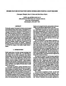
x ∈ Rn

PCA

Rd PCA

Search for dopt d : 1 → dmax d Avg. Error y ∈ R Feature Quadratic Rate Extractor Classifier

Fig. 1. Experimental setup.

(13)



1

Label (a) (b) (c) (d) (e) (f) (g) (h)

where T = T Σ − 2 , and the rows of T are selected as the d most significant eigenvectors of SH in (12). WLSS is not based on normalization with respect to a specific class parameters and hence its solution is not biased as the CLSS solution. Also, compared to the Chernoff method [4], WLSS formulation is much simpler and does not require the calculation of inverses and logarithms of the pairwise average covariance matrices. Furthermore, the calculation of calculaSH is O(C) which is faster than the corresponding   tion for the Chernoff method, which is O C 2 . Finally, unlike CLSS and the Chernoff method, WLSS does not rely on the non-singularity of the individual class covariance matrices and only their average is required to be non-singular. This makes WLSS a feasible feature extractor even for the cases where the small sample size yields singular estimated covariances. In the homoscedastic case where Σi = Σ, SH in (12) simplifies to C    Sh = P (ωi )μi μi T . (14) i=1

The rank of Sh is at most C − 1. Therefore, the minimum dimension for the linear SS does not exceed C − 1 for the homoscedastic case. Furthermore, Sh in (14) equals the between-class scatter matrix in the whitened space. Therefore, in the homoscedastic case, the solutions of WLSS and LDA coincide and WLSS can be considered as a heteroscedastic extension of LDA. Although it has been known that LDA provides an SS for the homoscedastic data [9], its equivalence to the homoscedastic WLSS proves that LDA provides a weighted least squares approximation of an orthonormal minimal-dimension linear SS in the whitened space.

2220

4. SIMULATION RESULTS The simulations compare the classification performance on the heteroscedastic data using the following non-iterative supervised linear feature extractors: LDA, Chernoff method [4], Mahalanobis method [5], CLSS [7], and WLSS. All of these methods are based on the first two central moments of the data. Accordingly, the data distributions are assumed Gaussian and the Bayes classifier with a quadratic rule is used. To facilitate the comparison, an experimental setup similar to [4] is assumed. UCI classification data sets [10] with more than 250 samples are used and their specifications are given in Table 1. The experiment on each data set is repeated 100 times and the average error rate (AER) over all the repetitions is calculated. In each repetition, the data set samples are split into %10 testing samples and %90 training samples used for the maximum likelihood estimation of the class means and covariances. Before any supervised feature extraction, a PCA projection is applied on the data which rejects all the eigenvectors with eigenvalues smaller than %0.0001 of the total variance (Fig. 1). This guarantees the non-singularity of the covariance estimates used by the quadratic classifier. AER for the PCA features is reported in the first column of Table 2. The feature extractors are then applied separately on the PCA transformed data. None of the methods specifies the number of features (d). Thus, the optimal number (dopt ) is calculated empirically. The minimum AER for each method over all the possible values of d is found. This AER and the minimizing dimension (dopt ) are used in Table 2 to compare the best results of the different methods. For each data set in Table 2, the AER values with no significant difference from the smallest value are boldfaced. The significance is decided according to the signed ranked test [11] with the significance level of 0.01. All the columns for

DB (a) (b) (c) (d) (e) (f) (g) (h)

PCA AER 0.3549 0.3126 0.3371 0.1504 0.6536 0.2582 0.1424 0.3133

LDA AER (dopt ) 0.0285 1 0.3815 1 0.2418 1 0.0534 1 0.5136 4 0.2635 1 0.1424 10 0.2247 3

Mahalanobis AER (dopt ) 0.0281 1 0.3788 1 0.2467 1 0.0586 1 0.4554 7 0.2471 1 0.1424 10 0.2332 3

CLSS AER (dopt ) 0.3507 5 0.3124 5 0.2843 2 0.1504 5 0.4925 11 0.2559 1 0.1424 10 0.3133 34

Chernoff AER (dopt ) 0.0273 1 0.3126 6 0.2403 1 0.0709 1 0.5439 13 0.2162 2 0.1424 10 0.2281 3

WLSS AER (dopt ) 0.0272 1 0.3126 6 0.2437 1 0.0602 1 0.4539 11 0.1774 5 0.1424 10 0.3129 6

Table 2. The average error rate (AER) and the optimal dimension (dopt ) for different feature extractors. data set (g) are boldfaced because all dopt values equal d PCA and all feature spaces coincide with the PCA space. From Table 2, the supervised feature extractors help to decrease AER or at least the required dimensionality in most cases. Although LDA yields a generally lower target dimensionality, the AER values for the heteroscedastic methods is generally lower because they use the second order information and the number of their features is not limited to C − 1. LDA exceptionally overcomes the other methods for data sets (d) and (h); but this alludes to nearly homoscedastic distributions for these data sets. Among the heteroscedastic methods, the best overall performance belongs to WLSS. Data sets (e) and (f) suggest WLSS as the best feature extractor with a significant margin. WLSS is among the significantly top methods for 5 data sets. The next top ranked method is the Chernoff method with significant success for 4 data sets. However, it requires several matrix operations including matrix logarithms for each class pair [4]. The average CPU time for the calculation of the scatter matrices from the available class parameters and the subsequent eigen-decomposition was calculated on a fixed workstation. The result is approximately 0.36s for the Chernoff method and in the range of 1.3ms to 1.8ms for WLSS and the other methods. Thus, WLSS provides a generally superior performance to the Chernoff method while requiring much lower computational load. 5. CONCLUDING REMARKS The proposed WLSS method is a non-iterative Bayes-errorbased feature extractor. As a linear operator, it preserves data Gaussianity and is computationally efficient for high dimensional data. WLSS utilizes the discriminative information in both first and second central moments of the data and there is practically no restriction on its feature space dimensionality. Furthermore, its simple formulation accounts for a very low computational requirement and a high generalizability. Also, LDA is derived as the special homoscedastic case of WLSS and hence as an approximation of a sufficient statistic in the whitened space. Moreover, the heteroscedastic SH formulation for WLSS is similar to the between-class scatter matrix in the whitened space. Therefore, enhancements such

2221

as weighted LDA, fractional-step LDA, and regularized LDA can be applied to WLSS as well. 6. REFERENCES [1] K. Fukunaga, Introduction to Statistical Pattern Recognition, Academic Press, second edition, 1990. [2] M. El Ayadi, M.S. Kamel, and F. Karray, “Toward a tight upper bound for the error probability of the binary Gaussian classification problem,” Pattern Recognition, vol. 41, no. 6, pp. 2120–2132, 2008. [3] G. Saon and M. Padmanabhan, “Minimum Bayes error feature selection for continuous speech recognition,” in NIPS, 2000, pp. 800–806. [4] R.P.W. Duin and M. Loog, “Linear dimensionality reduction via a heteroscedastic extension of LDA: the Chernoff criterion,” IEEE Trans. Pattern Anal. Mach. Intell., vol. 26, no. 6, pp. 732–739, 2004. [5] H. Brunzell and J. Eriksson, “Feature reduction for classification of multidimensional data,” Pattern Recognition, vol. 33, no. 10, pp. 1741 – 1748, 2000. [6] L. Devroye, L. Gy¨orfi, and G. Lugosi, A Probabilistic Theory of Pattern Recognition, Springer, 1996. [7] J.D. Tubbs, W.A. Coberly, and D.M. Young, “Linear dimension reduction and Bayes classification with unknown population parameters,” Pattern Recognition, vol. 15, no. 3, pp. 167–172, 1982. [8] B.C. Peters, Jr., R. Redner, and H.P. Decell, Jr., “Characterizations of linear sufficient statistics,” Sankhy¯a, Ser. A, vol. 40, pp. 303–309, 1978. [9] O.C. Hamsici and A.M. Martinez, “Bayes optimality in linear discriminant analysis,” IEEE Trans. Pattern Anal. Mach. Intell., vol. 30, 2008. [10] A. Asuncion and D.J. Newman, “UCI machine learning repository,” 2007. [11] J.A. Rice, Mathematical Statistics and Data Analysis, Duxbury Press, second edition, 1995.