Linear Parameter Varying Approach to Wind ... - Semantic Scholar

Linear Parameter Varying Approach to Wind Turbine Control Vedran Bobanac University of Zagreb Faculty of Electrical Engineering and Computing Unska 3, HR-10000 Zagreb, Croatia E-mail: [email protected] Abstract—Design of linear parameter varying control (LPV) for wind turbines is considered in this paper. Multivariable, robust control law, which can guarantee stability and desired performance in the whole operating region of the wind turbine, is obtained. LPV controller is compared with a classical controller. Keywords—wind turbine, linear parameter varying control, robust control.

I. INTRODUCTION Modern wind turbines are complex systems which are expected to operate autonomously and produce energy in a variety of operating conditions specified in the first place by the wind speed. Designing control system of a wind turbine is a challenging task as there are many conflicting requirements which should be taken into account. Foremost there is highly nonlinear relation between power in the wind and the wind speed. Wind power is proportional to the third power of the wind speed [8] and this nonlinearity reflects directly to the control system. Interaction of the wind and of the turbine blades causes torque which drives the rotor, but it also causes thrust on the rotor which is undesirable, as thrust causes structural loads and vibrations of tower and blades. Thrust on the rotor is very dependent on the pitching control strategy. Inadequately designed control may cause large tower oscillations and in the worst case can lead to the destruction of the turbine. On the other hand, by using advanced control techniques tower vibrations can be damped and the lifetime of the wind turbine can be extended. Moreover, the starting investment can be reduced because the construction of the turbine can be made lighter (lesser consumption of material) owing to the reduced structural vibrations. There are many other problems that make the design of the control system more demanding. Some of this problems are: stochastic nature of the wind, wind shear effect, tower shadow effect, wake effect in wind parks, the fact that it is impossible to measure the wind speed precisely enough to include the measured signal in the control system and so on. Wind energy industry is growing rapidly and new wind turbines are built larger and larger. As dimensions of wind turbines increase problems like tower and blade oscillations become more pronounced and designing the control system becomes more challenging. Therefore, it makes sense to explore applicability of the advanced control algorithms to the wind turbines. In recent years there has been a lot of research activity in this field. One

of the advanced control methods, called Linear Parameter Varying (LPV) control is the topic of this paper. The paper is organized as follows. In section II control objectives for modern wind turbines are given and in section III wind turbine mathematical model is described. Linear parameter varying control basics are given in section IV, while the algorithm for controller synthesis is described in section V. This section is followed by a presentation of simulation results in section VI. Conclusions are given in section VII. II. CONTROL OBJECTIVES Nonlinear relation between power in the wind and the wind speed has resulted in modern wind turbines having two main operating regions: below rated wind speed and above rated wind speed. Rated wind speed is defined as the lowest wind speed at which wind turbine may operate continuously at its rated power. Below rated wind speed, power that can be extracted from the wind is smaller than the rated power of the wind turbine and the control objective in this region is to maximize the energy conversion efficiency. Control is performed by adjusting the generator torque, while the pitch angle is kept around minimal value of 0o so that system is operating along maximum power coefficient curve [8]. Controlling the generator torque is possible because modern generators are not connected to the grid directly, but over the AC-DC-AC converter which allows generator speed to be varied in a wide range. Wind turbines, with synchronous generator that is connected to the frequency converter of rated generator power, are particularly suitable for such control strategy. Control of such wind turbines is considered in this paper. Above rated wind speed, power that can be extracted from the wind grows rapidly with the wind speed and it is greater than the rated power of the wind turbine. Control objective in this region is limitation of the turbine rotational speed to its rated value which implies that the wind turbine is operating at the rated power. This is the case because generator torque is kept at the rated value above rated wind speed, and it is well known that the electrical power is a product of generator torque and rotational speed. Control in this region is performed by pitching the turbine blades around their longitudinal axis which changes aerodynamic characteristic of the blades and therefore lowers energy conversion efficiency. This degradation in energy conversion efficiency is necessary as the wind turbine generator cannot operate continuously above its rated power.

Fig. 1. Classical wind turbine control system

Usual (classical) configuration of the wind turbine controllers is the following (Fig. 1): Below rated wind speed torque reference is usually generated by multiplying the square of the measured rotational speed with the optimal mode gain which results in maximal energy conversion efficiency [2,5,8]. In addition PI controller is used on the borders of operating region below rated wind speed as described in [8]. Above rated wind speed PI controller with gain scheduling is used. Gain scheduling is necessary because of previously mentioned plant nonlinearity [8]. III. MATHEMATICAL MODEL Physical phenomena that occur during aerodynamic conversion of wind energy into mechanical energy of wind turbine rotation are very complex and to describe them a complex mathematical model is required. Usual modeling method for describing this phenomena is called Blade Element and Momentum Theory and professional software tools for simulating wind turbines, such as GH Bladed, are based on this model [3]. This model uses implicit relations which are solved by using numerical methods, while the model deduction is based on combination of two approaches: actuator disk model and blade element theory. First approach observes wind turbine rotor as a solid disk and analyses its influence on free circulation of air, while the other approach observes each blade as series of infinitesimal segments and analyses aerodynamic phenomena on them. However the above described model is not directly applicable in design of the wind turbine control system, mainly because of implicit relations that it uses. That is the reason why a simpler, nonlinear mathematical model of the wind turbine is derived. For analyzing control strategy proposed in this paper a modern 1 MW wind turbine was modeled. The nonlinear model is implemented in Matlab/Simulink and is given by the following relations [8]: J t ωɺ = Ta − Tg 1 2 Ta = ρ a R3π CQ ( λ , β ) ⋅ ( vwind − xɺt ) 2 . 1 2 2 Ft = ρa R π Ct ( λ , β ) ⋅ ( vwind − xɺt ) 2 Ft = Mxɺɺt + Dxɺt + Cxt

(1)

Equations (1) describe wind turbine rotor dynamics, rotor torque, thrust on the rotor and equivalent tower dynamics, respectively. ω denotes rotational speed of the turbine rotor and for the considered wind turbine its rated value is 27 rpm. vwind denotes the effective velocity of the wind, but will be reffered to as simply “wind speed” in the sequel. Rated wind speed, at which rated power of 1 MW is achieved, equals 11 m/s. Cut-in wind speed of the wind turbine is 2.5 m/s, while cut-out wind speed is 25 m/s. Tg denotes generator reaction torque which has rated value of 3.54·105 Nm. Wind blowing over the turbine rotor causes aerodynamic torque Ta and thrust force on the rotor Ft. xt denotes tower top displacement caused by the thrust force. β is pitch angle of the turbine blades. Optimal pitch angle equals 0o, while at higher wind speeds (above rated) pitch angle can reach values up to 30o. Parameters λ, CQ and Ct are called blade tip to wind speed ratio, torque coefficient and thrust coefficient, respectively. CQ and Ct are nonlinear functions of λ and β. Jt denotes moment of inertia of the turbine rotor and ρa is air density which amounts 1.225 kg/m3. M, D and C denote tower modal mass, modal damping and modal stiffness, respectively. Blades are 28.7 meters long which is denoted with R. Even though tower height is not a model parameter, it is worth mentioning that the tower is 60 meters high. Drive train flexibility was not modeled because a wind turbine of interest has a synchronous generator with direct drive and it is a reasonable assumption that flexibility in the drive train is not very expressed [8]. Also, the effects of wind shear and tower shadow are not included in [1]. A family of linear models, which represents the basis for designing the control system, can be derived from the nonlinear model by linearization around series of operating points. A linear model (defined by the operating point) is given by the following relations: J t sω ( s ) = M a ( s ) − M g ( s ) M a ( s ) = M v′ vwind ( s ) − sxt ( s )  + M β′ β ( s ) + M ω′ ω ( s )

( Ms

2

)

+ Ds + C xt ( s ) = Ft ( s )

,(2)

Ft ( s ) = Fv′  vwind ( s ) − sxt ( s )  + Fβ′ β ( s ) + Fω′ ω ( s )

where Mv', Mβ', Mω', Fv', Fβ' and Fω' stand for partial derivatives. For every operating point, which is defined by the wind speed, a plant representation in form of (2) can be derived. Servo control system for pitching the turbine blades (control loop with servo drives, servo controllers and sensors for pitch angle measurement) are modeled as a second-order transfer function:

Gservo ( s ) =

β (s) 1 . = 2 β ref ( s ) a2 ⋅ s + a1 ⋅ s + 1

(3)

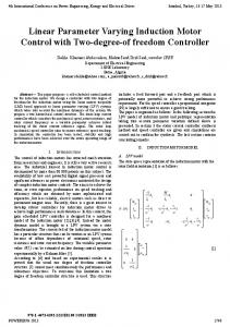
Principle scheme of the synchronous generator and the AC-DC-AC converter is shown in the Fig. 2. The variable-frequency AC from the generator is rectified to DC and then fed into the grid via grid side converter (AC inverter). Grid side converter is maintaining the DC voltage to a previously fixed value by using PI controllers. Grid side converter also obtains the desired power factor. Generator side converter controls generator torque by using direct torque control.

∞

∞

T ∫ z (τ )z (τ ) dτ < γ ∫ w (τ )w (τ ) dτ . T

0

Fig. 2. Generator and the frequency converter

Generator and frequency converter have very fast dynamics and they can respond almost instantly (within one discretization step on a real turbine) to the change in reference given by the torque controller. Therefore they are modeled as a fast first-order transfer function:

Ggenerator ( s ) =

Tg ( s ) Tgref ( s )

=

1 , T1 ⋅ s + 1

(4)

where T1 may have value of approximately 20 ms. IV. LINEAR PARAMETER VARYING CONTROL LPV control is recent reformulation of classical gain scheduling method. LPV theory observes nonlinear or linear time varying system as a linear system, dynamics of which is dependent on time varying parameters. LPV system can be described in the state-space form as follows:

xɺ (t ) = A (θ (t ) ) x ( t ) + B (θ (t ) ) u (t ) y (t ) = C (θ (t ) ) x(t )

,

(5)

where A(θ), B(θ) and C(θ) are continuous functions of a vector of time varying parameters θ(t). One of the shortcomings of the classical gain scheduling design is the lack of stability and performance guarantees of the nonlinear or time-varying closed-loop system. Unlike classical gain scheduling, LPV control algorithm can take into account arbitrary fast rate of variation of the scheduling variables and therefore it can guarantee stability and performance. In addition LPV controller is multivariable which allows more advanced control algorithms to be used than with classical SISO PI controllers. LPV open-loop model is obtained by linearising the nonlinear system around the set of equilibrium points. The family of linear systems is parameterized by the variables that define the operating point. In regular, power production operating condition, wind turbine is operating on the nominal trajectory, which means that all the process variables can be uniquely described by the wind speed. Thus, wind turbine LPV models are scheduled only by wind speed (θ(t)=vwind(t)). LPV controller is designed by a procedure similar to H∞ synthesis. Desired performance of the controller is specified by selecting performance channels (outputs and inputs) and associated weighting functions [14]. Algorithm minimizes the norm of the transfer matrix from performance input (disturbance, denoted w) to performance output (error, denoted z). It is said that the LPV system has the performance level γ if the following relation holds:

2

(6)

0

An alternative approach to H∞ problem is used where usual Riccati equations are replaced by Riccati inequalities which can then be written as linear matrix inequalities (LMIs) [7]. Therefore controller design can be formulated as a convex optimization problem with linear matrix inequalities (LMIs), which can be efficiently solved by using numerical algorithms, such as interiorpoint methods. The above performance specification requires the controller to be designed for each possible operating point defined by the scheduling variable. This implies solving an optimization problem with an infinite number of LMIs. Naturally, this is not possible in practice, so some methods have been derived to reduce the problem to one having a finite number of LMIs. In the case where plant matrices depend on the scheduling variables affinely it suffices to solve LMIs at the vertices of the polytope covering all the possible values of scheduling variables [1,2]. Unfortunately, plant matrices of the wind turbine model of interest don't depend on the wind speed affinely, at least not in the whole operating region of the turbine. Therefore alternative approach called gridding is used [2,10]. This is an approximate method, but still with the assumption of arbitrary fast parameter variation. Idea of this method is to design a LPV subcontrollers only in operating points between which affine parameter dependency of the plant matrices on the scheduling variables can be assumed. It is important that the grid is chosen dense enough to catch all the nonlinearities in the system. On the other hand having lot of grid points will cause heavy computational effort, so the trade-off between these two objectives must be considered when choosing the number of grid points.

V. CONTROLLER SYNTHESIS The procedure for designing an LPV controller is given in the following steps: 1. Select k grid points (operating points) by observing nonlinear plant parameters in dependency on the scheduling variable θ. 2. Linearise the nonlinear plant model around the selected grid points to obtain k linear plant models in the statespace form. 3. Select performance channels and weighting functions. 4. Include the weighting functions in the linear plant state-space models to obtain the augmented plants. 5. Solve a semidefinite program consisting of 2k+1 LMIs to obtain the performance level γ and matrices R and S (which define the Lyapunov matrix Xcl). Matrices R and S must be the same for every chosen grid point (algorithm is given in [1,7]). 6. Obtain the subcontroller matrices, for each chosen grid point, by the algorithm described in [6]. 7. Connect obtained subcontrollers by linear interpolation in dependency on the scheduling variable θ.

eω

We(s)

e~ω βref

Tgref vwind

vwind

eω

y

u

Tgref

Tg

PITCH SERVO EQUIVALENT SUBSYTEM

β

xt

gref

z

WX(s)

~ xt

Gx_Tg(s) GTg(s) Gx_β(s) - -

- -

βref

GENERATOR + FREQUENCY CONVERTER

- -

- -

-

-

ωref -

WT(s)

T~

Gx_v(s) Gv(s)

w

ω

Gβ(s) WIND TURBINE (LINEARISED)

Rotor speed measurement

Fig. 3. Augmented plant for single operating point

Linearised plant model is obtained as described in section III of this paper. By selecting performance channels and weighting functions the desired behaviour of the closed loop control system is specified. Augmented plant used for designing the LPV controller in this paper is shown in Fig. 3, where Gv , Gxɺ _ v , GTg , Gxɺ _ Tg , Gβ and

Gxɺ _ β denote linearised transfer functions from wind speed, generator torque and blade pitch angle to tower top velocity and rotational speed of the turbine. Weighting functions are given by following relations: We =

s / M β + ωβ

s / M e + ωe ; Wβ = ; s + ωe ⋅ Ae s + ωβ ⋅ Aβ

WT =

s / M T + ωT ; WX = M X . s + ωT ⋅ AT

(7)

Parameters of weighting functions are chosen depending on the grid point. Augmented plant from Fig. 3 can be written in the state-space form with two inputs and two outputs as follows:

xɺ (t ) = Ai ⋅ x(t ) + B1i ⋅ w(t ) + B2i ⋅ u (t ) z (t ) = C1i ⋅ x(t ) + D11i ⋅ w(t ) + D12i ⋅ u (t ) , i = 1...k . (8) y (t ) = C2i ⋅ x(t ) + D21i ⋅ w(t ) + D22i ⋅ u (t )

NS  0 

T RC1Ti B1i  T  Ai R + RAi 0   N ⋅  C1i R −γ I D11i  ⋅  R  I    0 T B1Ti D11 −γ I  i  < 0, i = 1,..., k

 AiT S + SAi SB1i C1Ti    NS 0  T ⋅  B1Ti S −γ I D11 i⋅  I   0 D11i −γ I    C1i  < 0, i = 1,..., k T

(11)

where NR and NS denote orthonormal bases of the null spaces of (B2T,D12T) and (C2,D21) respectively. A semidefinite program can now be formulated, with γ as an objective function and the above LMIs as constraints. This is a convex optimization problem and it can be solved by using one of the available solvers. In this paper Sedumi, solver for linear, quadratic and semidefinite programs, was used. By solving this program matrices R, S and performance level γ are obtained. Next step is to compute k subcontrollers which correspond to the selected grid points. This is done by using explicit controller formulas, along the lines of [6]. Obtained family of subcontrollers can be written as:

xɺK (t ) = AKi ⋅ xK (t ) + BKi ⋅ y (t ) u (t ) = CKi ⋅ xK (t ) + DKi ⋅ y (t )

, i = 1...k .

0 I  , (9)

0 I  , (10)

(12)

The alternative way of writing the subcontroller matrices, which will be used later, is given by:

A K i =  Ki  C Ki

BKi  , DKi 

i = 1,..., k .

(13)

In that case the controller used for any operating point (any wind speed) between the grid points can be obtained by a linear combination of the subcontrollers (12), with no violation of (6) [1,2,10]. Since LPV models are scheduled only on one variable (wind speed), controller for any operating point can be calculated from two subcontrollers, which correspond to the two neighbouring grid points. Of course, information about the current operating point must be accessible as well. This information is provided by estimating the wind speed [8,17], so the following convex decomposition can be written:

vˆwind = α1 ⋅ vi + α 2 ⋅ vi +1 ,

α1 + α 2 = 1, α1 , α 2 > 0, i = 1,..., k − 1,

Variables w, z, y and u, which are also marked in Fig. 3, represent performance input, performance output, controller input and controller output, respectively. Ai, B1i, B2i, C1i, C2i, D11i, D12i, D21i and D22i are constant matrices for grid point i, while k is the number of grid points. Along the lines of [1], there exists an LPV controller guaranteeing stability and H∞ performance level γ if and only if there exist two symmetric matrices R and S which satisfy the following system of 2k+1 LMIs:

NR  0 

R I   I S ≥ 0 ,  

β~ ref

Wβ(s)

(14)

vi ≤ vˆwind ≤ vi +1 , where vˆwind is the estimated wind speed and vi , vi +1 are wind speeds which define the grid points. The above convex decomposition gives factors α from which controller for the current operating point can be calculated as:

K (vˆwind ) = α1 ⋅ K i + α 2 ⋅ K i +1 .

(15)

This approach may be conservative since Lyapunov matrix Xcl (defined by matrices R and S) is the same for all grid points, but on the other hand stability and performance can be guaranteed in the whole operating region of the turbine, for arbitrary fast parameter variation and for large input signals. Configuration of the LPV wind turbine control system is shown in Fig. 4.

Fig. 4. LPV wind turbine control system

VI. SIMULATION RESULTS Algorithm described in the previous section has been applied for the design of an LPV controller for the considered wind turbine. Controller parameters were calculated for five grid points defined by wind speeds: 4 m/s (near cut-in wind speed), 9 m/s, 10 m/s (wind speeds just below rated), 12 m/s (wind speed just above rated) and 25 m/s (cut-out wind speed). Plant parameter dependency on the scheduling variable (wind speed) between these grid points can be approximated by the affine functions. Simulations were carried out in Matlab/Simulink for the whole operating region of the wind turbine (wind speeds from 3 to 25 m/s) with the wind speed stepwise changes of 1 or 2 m/s. This form of the wind never occurs in the nature, but it can be very useful to gain insight into the control system dynamic behaviour. Results of the simulations are shown in figures 5, 6 and 7 for the wind speeds below rated, around rated and above rated respectively. Figures show the wind speed for which the simulation has been conducted and the relating system responses. On the right side of the figures, enlarged graphs, for one segment of the simulation, are shown. Responses are plotted in the following order: rotational speed of the turbine, pitch angle of the blades (or the tip speed ratio), generator torque and tower top displacement. LPV controller is compared with a classical controller which uses the control strategy described in section II of this paper. LPV controller is multivariable which means that it uses both pitch angle and generator torque to control the rotational speed. Generator torque may be increased over the rated value for the short period of time as described in [8], where the use of generator torque for compensating wind gusts has been proposed. For the operating region below rated wind speed LPV controller was tuned so that similar behaviour to the classical controller is achieved. This can be seen from the responses in Fig. 5. Main control objective in this operating region is maximization of energy conversion efficiency and this is obtained by maintaining the tip speed ratio at the optimal value of 7.9, for as long as possible. The biggest difference to the classical controller can be seen in the generator torque control signal. This happens due to different control strategy in the operating region below rated wind speed. Classical control strategy multiplies the square of the measured rotational speed with the optimal mode gain and feeds the result to the frequency converter. On the other hand LPV controller

uses standard feedback control configuration where the rotational speed measured error (the difference between the reference and the measured output) is input to the LPV controller which produces the signal for the frequency converter. LPV controller for the operating region below rated wind speed was designed with the trade-off between frequency converter activity and the time that system spends at the optimal tip speed ratio. Tip speed ratio could have optimal value for a longer period of time than it is shown in Fig. 5, but this would be on account of more variations in the generator torque and thus increased loading of frequency converter. Below rated wind speed the blade pitching system shouldn't be active and this was achieved by awarding large gain to the Wβ weighting function. Blade pitch angle has a constant value of 0o in this operating region and that is why pitch angle responses are not shown in Fig. 5. This is also the reason why tower top displacement responses in Fig. 5 are very similar, since pitching control strategy has a dominant effect on tower oscillations. Operating region around rated wind speed is very challenging and demanding from the control point of view. In classical control configuration this is the region where switching between torque and pitch controllers occurs. This can have negative impacts on the turbine rotational speed and tower oscillations, especially in the case of large wind gusts. By using method proposed in this paper problems connected with switching between torque and pitch controllers are avoided since only one multivariable controller is used and the only thing that changes are controller parameters. Simulation results for the operating region around rated wind speed are shown in Fig. 6. Blade pitch angle is plotted instead of tip speed ratio, since maintaining the optimal tip speed ratio is of interest only below rated wind speed. LPV controller for the operating region around rated wind speed was designed so that more variation in generator torque is allowed while saving the pitch servo drive. This is desirable because pitch servo drive is one of the vital components of the modern wind turbines, but also one of the components with the shortest lifetime as it wears out quickly. Reducing pitch activity also has a positive impact on the tower oscillations, since all the changes in the pitch angle reflect directly on the tower thrust force and thus the tower nodding. From Fig. 6 it can also be seen that the wind turbine rotational speed control is significantly improved by using LPV controller. Simulation for the operating region above rated wind speed gave similar results as for the wind speeds around rated. From Fig. 7 it can be seen that the improvement in the control of rotational speed has been achieved, together with the reduction of the pitch activity and reduction of the tower oscillations. Great help in achieving this performance improvements is strategy of using generator torque for compensating wind gusts. If, for some reason, it is necessary to change performance demands on the controller, it can be done by altering weighting functions given by the expressions (7) and recalculating parameters of the LPV controller. For example, if reduction of frequency converter activity is necessary, it can be achieved by awarding more weight on the generator torque weighting function WT.

Fig. 5. Simulation results below rated wind speed

VII. CONCLUSION LPV controller was successfully implemented and simulations have given satisfactory results. Improvement regarding to classical controller design has been achieved. Strength of the proposed method lies in a fact that different weight can be assigned to particular objectives. For example higher damping of structural vibrations can be obtained by allowing more variations in the control signal. This is done by selecting appropriate weighting functions. Another advantage of this method is that a single controller can be used in the whole operating region of the wind turbine, so there is no need for switching the controllers. This also improves system behaviour on the edge of the operating regions, i.e. around rated wind

speed. Moreover, the resulting controller is multivariable which allows more flexibility in designing the control algorithm. VIII. FUTURE WORK So far, simulations with LPV controller have been carried out only in Matlab/Simulink, on a simplified model. Future work will encompass extensive simulations in the professional tool GH Bladed where the impact of the LPV control strategy on various wind turbine variables can be investigated. Besides in GH Bladed, LPV control strategy will also be tested in the newly built Laboratory for renewable energy sources (LARES) at the Faculty of Electrical Engineering and Computing,

Fig. 6. Simulation results around rated wind speed

University of Zagreb, Croatia. Testing on a laboratory wind turbine is important because the impact of all the problems present on real systems (nonlinearities, measurement noise, sensitivity to disturbances etc.) can be investigated. This is one step closer to the final goal which is implementation of the LPV control algorithm on real MW-class wind turbines. Results presented in this paper include only simulation responses in time domain, but the main idea of the proposed method is to provide control law which is robust against disturbances and plant parameter uncertainty. Therefore, further research will also encompass investigation of the LPV controller robustness and its comparison to the robustness of the classical control strategies.

REFERENCES [1]

[2]

[3] [4]

[5]

P. Apkarian, P. Gahinet, G. Becker, Self-scheduled H∞ Control of Linear Parameter-varying Systems: a Design Example, Automatica, 1995; 31(9):1251–1261. DOI: 10.1016/00051098(95)00038-X F.D. Bianchi, H. De Battista, R.J. Mantz, Wind Turbine Control Systems – Principles, Modelling and Gain Scheduling Design, Springer-Verlag, 2007. E.A. Bossanyi, D.C. Quarton, GH Bladed – Theory Manual, 282/BR/009, Garrad Hassan and Partners Limited, 2003. E.A. Bossanyi, D. Witcher, D.C. Quarton, GH Bladed Version 3.65 – User Manual, 282/BR/010, Garrad Hassan and Partners Limited, 2004. T. Burton, D. Sharpe, N. Jenkins, E. Bossanyi, Wind Energy Handbook, John Wiley & sons, Chichester, UK, 2001.

Fig. 7. Simulation results above rated wind speed [6]

P. Gahinet, Explicit Controller Formulas for LMI-based H∞ Synthesis, Automatica, 1996; 32(7):1007–1014. DOI: 10.1016/0005-1098(96)00033-7 [7] P. Gahinet, P. Apkarian, A Linear Matrix Inequality Approach to H∞ Control, International Journal of Robust and Nonlinear Control, 1994; 4:421–448. DOI: 10.1002/rnc.4590040403 [8] M. Jelavić, N. Perić, Wind Turbine Control for Highly Turbulent Winds, Automatika, Vol. 50, No. 3-4, December 2009. [9] K.Z. Østergaard, Robust, Gain-Scheduled Control of Wind Turbines, PhD thesis, Aalborg University, 2008. [10] K.Z. Østergaard, J. Stoustrup, P. Brath, Linear parameter varying control of wind turbines covering both partial load and full load conditions, International Journal of Robust and Nonlinear Control, 2009; 19:92–116. DOI: 10.1002/rnc.1340 [11] N. Perić, Automatic Control (in Croatian), Lectures, Faculty of Electrical Engineering and Computing, Zagreb, 2005. [12] I. Polik, Addendum to the Sedumi User Guide Version 1.1, McMaster University, 2005.

[13] C. Scherer, P. Gahinet, M. Chilali, Multiobjective OutputFeedback Control via LMI Optimization, IEEE Transactions on Automatic Control, 1997; 42(7):896–911 [14] S. Skogestad, I. Postlethwaite, Multivariable Feedback Control, John Wiley & Sons, Chichester, UK, 1996. [15] V. Spudić, Appliance of Semidefinite Programming to Identification, Analyses and Synthesis of the Control System (in Croatian), Masters thesis, Faculty of Electrical Engineering and Computing, Zagreb, 2007. [16] J.F. Sturm, Using Sedumi 1.02. a Matlab Toolbox for Optimization over Symmetric Cones (Updated for Version 1.05), Department of Econometrics, Tilburg University, Netherlands, 2001. [17] I. Tibinac, Wind Turbine Robust Control (in Croatian), Masters thesis, Faculty of Electrical Engineering and Computing, Zagreb, 2009. [18] Z. Vukić, Lj. Kuljača, Automatic Control (in Croatian), Kigen, Zagreb, 2005. [19] K. Zhou, J. Doyle, K. Glover, Robust and Optimal Control, Prentice-Hall, Englewood Cliffs, USA, 1996.