The Effects of Varying Parameter Values and Heterogeneity in an Individual-Based Model of Predator-Prey Interaction William J. Chivers ab and Ric D. Herberta a
Faculty of Science and Information Technology, The University of Newcastle, PO Box 127, Ourimbah, NSW 2258, Australia (
[email protected] and
[email protected]) b
Corresponding author
Abstract: An individual-based model which produces non-linear predator-prey dynamics is described. The importance of individual variation to the stability of the population dynamics predicted and the advantages of the individual-based approach to modelling ecological systems are discussed. The individual-based model is compared with the traditional approach of population ecology—the modelling of populations with state variable equations. The individual-based model built here produces similar patterns of mutual dependence of the populations to those produced by the state variable model but has additional utility. It greatly simplifies the adjustment of individual environmental parameters which may be built into the model and it makes it possible to follow individuals or individual parameter values through the simulation. The cost of the utility of the individual-based approach is in the complexity of the model itself, which is more difficult to build than many state variable models. A common finding in the literature of individual-based modelling in ecology is the importance of individual variation. The individual-based model described here is built with a minimum of biological complexity, but still we find that individual variation in the model has profound effects on the stability of the population levels over long time periods. Keywords: Individual-based modelling, Lotka-Volterra equations, State variable modelling.
1
INTRODUCTION
The use of individual-based modelling in ecology has grown rapidly since the pioneering work of DeAngelis et al. [1979], Kaiser [1979] and Łomnicki [1978] in the modelling of systems characterized by large numbers of discrete elements [DeAngelis et al., 2001; Grimm, 1999; Judson, 1994; Łomnicki, 1999]. Individual-based modelling is an alternative to the more traditional state variable approach in which ordinary or partial differential equations are used to predict system outcomes over time. The motivations for building individualbased models include looking for a mechanistic understanding of the complex interactions in ecological systems, the need to build a predictive tool to be used to forecast population levels and an exploration of the effect of adding complexity to a model
in order to introduce biological realism [DeAngelis et al., 2001; Huston et al., 1988]. An individual-based model consists of a set of heterogeneous discrete objects which change their state over time in a changing environment. Execution of the model is effected by simulating local interactions between individuals and the time-varying, heterogeneous environment. In contrast, the traditional state variable modelling takes a top-down approach, seeking to express relationships between global outcomes. Global outcomes are modelled directly in a set of equations, and execution consists of evaluating the equations over time, often in discrete time intervals. Populations, rather than individuals, are modelled. Inherent in state variable models are simplifying as-
The state variable approach has been successful in providing general understanding of system dynamics [Bousquet, 2001], but it does not address issues of individual heterogeneity, individual learning and behaviour, local interactions or environmental heterogeneity which are important in modelling the complexity of these systems. Our empirical understanding of population dynamics and individual interactions is that these systems cannot easily be modelled using an equation-based state variable approach [DeAngelis et al., 2001; Huston et al., 1988; Łomnicki, 1999; Schmitz and Booth, 1997]. The individual-based approach seeks to address these problems. Individuals in an individual-based model have potentially unique state, behaviour and experiences. The behaviour of an individual depends on global rules of engagement and on the state and experience of the individual. The details of the interaction between individuals and the different experiences of the individuals can have a significant effect on the overall system dynamics and population levels, and begin to address the criticisms of the generalization of these factors in state variable models [DeAngelis et al., 2001; Schmitz and Booth, 1997]. In this paper we describe two models of the population dynamics of a predator species and a prey species. A state variable model which uses the Lotka-Volterra coupled differential equations is built and compared with an individual-based model. Both models describe the interaction of a prey species and a predator species. The individualbased model creates individuals with unique state, behaviour and experience and allows them to interact according to rules coded into the system. The Lotka-Volterra equations are a top-down view of the system in which individuals are not explicitly modelled. We use generalized species, meaning that some arbitrary decisions were made about the species. The individual-based model is built with a mini-
350
300
250
Population
sumptions such as homogeneity of individual properties, experiences and behaviour. Interactions typically occur randomly in one homogeneous environment space. There are, however, degrees of complexity in ecological systems including temporal and spatial scales, behavioral mechanisms and learning which are not easy to model in differential equations. The mathematics becomes intractable as the details or number of species rises [DeAngelis et al., 2001; Łomnicki, 1999; Schmitz and Booth, 1997].
200
150
100
Predators Prey 50
0
0.5
1
1.5
2 TimeUnit
2.5
3
3.5
4 5
x 10
Figure 1: The state variable model.
mum of biological complexity. Parameter values which result in stable cycling of population levels are found and the results of adjusting these parameter values are investigated. One modification is then introduced to explore the effects of adding further biological realism. The details of the individualbased model built here were inspired by the Gecko model as described by Schmitz and Booth [1997]. We find that the interaction of the individuals in the individual-based model generates comparable results to the state variable model—the population levels are interdependent and exhibit similar patterns. The advantages of the individual-based approach include relatively easy access to finely detailed parameters which are almost inaccessible in an equation-based approach. Perhaps most importantly, we find that the level of variation that exists among the individuals in the individual-based model has profound implications for the stability of the population levels predicted by the model. 2
THE STATE VARIABLE MODEL
The coupled set of differential equations developed by Lotka and Volterra in the 1920s (see, for example Adler [1998]) are used here to implement a state variable approach to modelling the population changes over time resulting from the interaction of a predator species and a prey species. The equations model the rate of growth of the prey as dependant on interactions with predators (the prey have unlimited resources such as food), and the rate of growth of the predators dependant on the availability of prey. The model is both parsimonious and deterministic.
The equations are: db(t) dt dp(t) dt
= [λ − ²p(t)]b(t)
(1)
= [−δ + ηb(t)]p(t)
(2)
Where b represents the population of prey, p the population of predators, λ the prey growth rate in the absence of predators, ² the chances of a prey object being eaten, δ the predator growth rate in the absence of prey and η the chances of a predator eating. The initial population levels are known. We use the Euler method to implement an ODE solver. Figure 1 is a graph of the data produced by a computational implementation of the ODE solver. The model is calibrated with the following parameter values: η = 0.006, ² = 0.0075, δ = 1.0 and λ = 1.2, and initial values: b0 = p0 = 100. The simulation was run for 40 time units with a time step of 0.0001. The assumptions on which the Lotka-Volterra model is based include the following: • The rate of growth in each population is a) constant relative to its own population size, and b) proportional to the other population size. • Prey never independently escape an encounter with predators: escape and hunting strategies are not modelled. • Homogeneous distribution of both species, which encounter each other at a rate proportional to the product of the two population sizes.
they represent is a problem if these individual environmental factors are important to the research being undertaken. While the assumptions can be manipulated by increasing the number of parameters and/or using partial differential equations, the resulting model is often complex and not easy to change [DeAngelis et al., 2001; Van Dyke Parunak et al., 1998]. The individual-based model built here makes some of the assumptions above, including the homogenous distribution of the species. In this model, however, system elements such as predator behaviour after a meal and prey resources are explored far more easily than would be possible with these coupled differential equations. 3
THE INDIVIDUAL-BASED MODEL
The individual-based model described here creates individual predators and prey, each with a potentially unique state. This state affects the behaviour of the individual in some of the implementations described below. Individuals maintain a resource total which is a simple analogy of the energy reserves stored by living animals. The concept of using resources as the currency of the model was inspired by the Gecko model of Schmitz and Booth [1997]. Each individual is given a resource level when it is born or created at the beginning of a simulation, and may add to the resource level by eating. Predators acquire the resources of their prey when they are eaten, and prey are given resources during each cycle of the simulation. A cycle is defined here as the basic time-step of the model and may represent different realistic time steps depending on the species being modelled.
• Predator behaviour is unchanged by a meal. • Prey have unlimited resources and grow exponentially in absence of predators. Their only cause of death is being eaten. • The predators have unlimited resources apart from food. • Only two species are interacting. These assumptions are intrinsic in the model and in the parameters, which represent many environmental factors and characteristics of the two species. They illustrate the tendency of state variable models to simplify and generalize system characteristics. The difficulty in mapping the four model parameters to the numerous environmental factors that
The individuals reproduce when they have enough resources or they may die of starvation or being eaten. Individuals attempt to make the most of their environment by collecting resources and reproducing. The environment created by the model at the start of a simulation changes as the individuals interact and the population levels change. The model is hierarchical in the sense that state and behaviour may be coded at the individual level or at the level of the environment. The model output is the population levels of the two species each cycle. Statistics may also be calculated and displayed. The basic model inputs are:
250
• Initial numbers of predators and prey • Predator chances of eating (to be multiplied by the prey population)
150 Population
• Initial resources of individuals of both species
200
• Reproductive cost for both species
100
• Metabolic tax per cycle for both species
50
• Maximum and minimum resources to be added to each prey individual per cycle
Predators Prey 0
0
50
100
150
200
250
Cycle
3.1 Description of Processing Per Cycle
Figure 2: The individual-based model
During each cycle of the simulator each predator and prey object is processed. The entire predator population is processed before the entire prey population. Processing the populations involves: 700
Each prey individual is given resources each cycle to simulate eating—whether the prey are herbivores or carnivores is not relevant to this model. The number of resources given to each prey individual is randomly selected from between an upper and lower bound—two of the model parameters. This is a source of variation between individuals in the prey and predator populations. Apply metabolic tax. A tax is deducted from the resource total of each individual to simulate the metabolic cost of living for each cycle. If the resource total drops below the metabolic tax per cycle, the individual dies and is removed, as it does not have the resources to live one more cycle. The predators do not eat those prey that have died of starvation. The tax for predators is higher than the tax for the prey, but these two parameters are global.
600
500 Population
Implement resource intake. Each predator is given a chance to eat once per cycle. Its chances of eating are proportional to the prey population, as in the Lotka-Volterra equations. If the predator is to eat, a prey individual is selected at random and removed from the simulation. The resource total of this prey individual is added to the resource total of the predator. The predators acquire all the resources of their prey, representing an unrealistic trophic efficiency of 100%—more realistic trophic efficiencies will be explored in future research. This model operates in one environment space, again like the Lotka-Volterra equations, so the prey eaten can be anywhere in the environment space.
400
300
200
100 Predators Prey 0
200
400
600
800
1000 1200 Cycle
1400
1600
1800
2000
Figure 3: The individual-based model over 2200 cycles
Process reproduction. Each individual may produce one offspring per cycle if it has enough resources to both reproduce and live one more cycle. If an individual is to reproduce, a reproductive tax is removed from its resource total to represent the cost of bearing offspring, and a new individual is added. The new individual is not processed until the next cycle. The individuals in this model reproduce by parthenogenesis—mating behaviour and its associated complexity is not modelled. The reproduction rate of the predators increases as the prey population increases and more resources are available. The metabolic costs of reproducing are global parameters.
14000
3.2 Simulating Population Dynamics with Individuals
The populations in Figure 2 appear to be dependent on each other as would be expected given the model algorithm. The predator population is dependant on the prey as a source of food, and the prey population is dependent on the predators as their chances of being eaten rises as the predator population rises. No statistical analysis was done to test this dependency. This particular set of parameters results in populations which cycle indefinitely. Figure 3 illustrates the model output over 2200 cycles: we have run the simulator for over 100 000 cycles with similar results. Figure 3 is typical of the output over thousands of cycles using different sets of stable parameter values. The population levels of the two species demonstrate cycling levels as do the population levels of the Lotka-Volterra equations, but the stochastic and possibly chaotic nature of the model is evident in the varying overall population levels over many cycles. Because of the stochastic nature of the model, and because the model was sensitive to parameter values, a statistical analysis of population levels to accurately determine trends was not pursued. The figures presented in this paper are representative of the results—the model is not deterministic and so each execution results in a different output. It is worth noting an implementation detail here: the computer programming language used (Java) generates pseudorandom numbers using the linear congruential method [Arnold et al., 2000]. If the same seed is used to generate the pseudorandom numbers in different executions of the model, an identical sequence of pseudorandom numbers will result. This means that while the model has a stochastic element, an individual execution of the model may be exactly repeated, and the effects of altering parameter values may therefore be reliably tested.
10000
Population
Once the model was built we commenced a search of the parameter space to calibrate the model for stable cycling population levels after transient dynamics. The simulation stops if one population drops to zero. Stable combinations of parameters were quickly found, indicating that the model is inherently stable. As Figure 2 illustrates, the model output is similar to that of the Lotka-Volterra equations. The simulations graphed here were started with 40 predators and 80 prey and were executed for 250 cycles of the model unless otherwise noted. Population levels in Figure 2 have a mean of 70 predators and 110 prey.
12000
8000
6000
4000
2000 Predators Prey 0
0
5
10
15 Cycle
20
25
30
Figure 4: Prey population in the absence of predators
One test of the validity of this model is to execute it with only one of the species present. In the absence of predators, the prey population increases exponentially (Figure 4). Conversely, in the absence of prey the predators quickly become extinct as they use resources but cannot replace them. These results are similar to those predicted by the state variable model. 4
THE EFFECTS OF VARYING PARAMETER VALUES
The reasons for developing individual-based models in ecology include the possibility of adjustment of individual states or behaviour and of access to parameters which are hidden in the small number of aggregated and generalized parameters characteristic of state variable equations. Here we access specific parameters to explore the effect of making small changes to them. 4.1
An Increase in the Prey Resources
The model is very sensitive to some, but not all, of the parameter values. Small increases in the metabolic tax, for example, quickly result in extinction of one or both species. Figure 5 illustrates the result of a small increase in the resources available to the prey. After 250 cycles the predator population mean is 112 and the prey population 117 compared with the figures 70 and 110 respectively in Figure 2. This set of parameters is also stable over thousands of cycles, and in fact displays less stochastic variation than is illustrated in Figure 3.
200
8000
7000
6000
150
Population
Population
5000
4000
3000
100 2000
1000 Predators Prey
Predators Prey 50
0
0
50
100
150
200
250
0
20
40
Cycle
Figure 5: An increase in prey resources
Predator Reproductive tax (Resource units 600 700 800
Predator mean
Prey mean
70 73 77
110 117 127
Table 1: Varying predator reproductive cost
60 Cycle
80
100
120
Figure 6: Predator reproductive tax of 890 resource units
Multiplicative parameter 0.90 0.95 1.00 1.05 1.10 1.15
Predator mean 104 73 90 89 89 89
Prey mean 1787 131 130 132 132 132
Table 2: Varying limits on predator satiation
4.2 An Increase In The Reproductive Cost To The Predators The sensitivity of this model to some parameter values is in contrast to its robustness to changes in other parameter values. The latter may be illustrated by adjusting the reproductive cost applied to the predators. One might initially expect that this would lower the predator numbers but the mean predator and prey numbers after 250 cycles were resistant to this change until the parameter value reached a critical value, where the population numbers become unstable (Table 1 and Figure 6). Below this figure, increasing the reproductive cost to the predators lowered the predator birth rate, but those remaining had greater food resources and therefore a lower death rate. 5
SIMULATION OF PREDATOR SATIATION
Predators in the individual-based model described above are given a chance to eat each cycle, and if given the chance to eat they will do so regardless of their existing resource level. That is, the model
does not take into account predator satiation. The first modification made to this model was to address this omission by preventing the predators from eating when their resource levels were above a given amount. This level was initially set at the sum of the costs of reproduction and metabolic tax of one cycle. We then tried making small adjustments to this level. Table 2 illustrates representative final population means after 100 cycles for various adjustments to the satiation level—the sum of the costs of reproduction and metabolic tax of one cycle is multiplied by the figure in the left column. A multiplicative parameter of 0.9 combined with a maximum of one prey per cycle restricts the predators’ access to prey too greatly, resulting in an exponentially increasing prey population (Figure 7). As the value of the parameter increases the prey population mean is reduced. A parameter value above 1.0 does not affect the population mean unless predators are allowed to eat more than one prey per cycle, in which case both populations are reduced as the predators eat too many prey. This is not illustrated
4
1000
x 10
2.5
Predators Prey Prey Resource SD
900
800
2 700
600
Population
Population
1.5
500
400
1 300
200
0.5 100
Predators Prey 0
0
10
0
20
30
40
50 Cycle
60
70
80
90
100
0
10
20
30
40
50 Cycle
60
70
80
90
100
Figure 9: Higher initial resource variation
Figure 7: A low predator satiation parameter
100
90
80
70
Population
60
50
40
30
20
10
0
Predators Prey Prey Resource SD 0
2
4
6
8
10
12
14
16
18
Cycle
Figure 8: Low initial resource variation
in this table as these results reflect the predators eating a maximum of one prey per cycle. 6
THE IMPORTANCE OF INDIVIDUAL VARIATION
While the model is robust to small changes in the reproductive cost to the predators below a given level, it is very sensitive to other parameters, such as the prey resources described above. The resources of each individual are the only source of individual variation in this model, and they are very important to the stability of the population numbers. If the simulator is started with little variation in the resource levels of the individuals, the population levels are very unstable and one of the populations quickly drops to zero. Figure 8 illustrates the two
populations and the standard deviation of the prey resources for each cycle when the resource standard deviation is low to begin with (predators: 128; prey: 74). The simulation lasts less than 20 cycles, when the predator population drops to zero and the simulation ends. The range of prey resource standard deviation values in this figure is 74–99. Figure 9 illustrates the simulation started with higher resource standard deviations (predators: 150; prey: 541), and is in fact the first 100 cycles of the simulation in Figure 2 with the standard deviation of the prey resources for each cycle added to the figure. The range of prey resource standard deviation values in this figure is 327–922. The importance of the level of variation in resources to the stability of the model over many cycles is consistently observed over the parameter space investigated. The initial prey resource variance is more important than the initial predator resource variance. It is difficult to make conclusions about the importance of this finding as the model is of two generalized species and the parameter values are therefore not derived from empirical data. We add this finding, however, to the growing evidence in the literature on individual-based modelling in ecology that individual variation is important to the long-term viability of species in these models [DeAngelis et al., 2001; Huston et al., 1988; Łomnicki, 1999; Schmitz and Booth, 1997]. The significance and importance of individual variation, and the correlation between the prey numbers and the prey resource standard deviations will be the subject of future research.
7
DISCUSSION
7.1 The Model Parameters A major difference between the individual-based approach and the state variable approach is the method by which the parameters are modelled. The number of parameters in an ecological system is large, but the traditional state variable approach tends to reduce these to a low number of generalized parameters. If the adjustment of individual parameters is not important to the model builder, then the small number of parameters of the state variable approach may be an advantage. Reducing the many natural parameters which affect a system to a few does, however, increase the difficulty in interpreting or adjusting these parameters. In contrast to the state variable approach, individual-based modelling has the potential to explicitly model every relevant parameter more easily than state variable modelling, facilitating the interpretation and adjustment of individual parameters. Builders of individual-based models should, however, endeavour to keep the number of parameters to a minimum as the addition of each parameter increases the complexity of the model, increasing the difficulty with which the model dynamics may be understood. Finding the critical parameters for the question at hand and modelling only these parameters is a significant challenge for individual-based modelling. The explicit modelling of critical parameters may facilitate direct experimentation with and verification of the model. For example, adjustment to the limits of predator satiation in the model described here leads to insight into the level of this parameter necessary for optimal population levels. The importance of making adjustments to specific parameters in some research is emphasized by Van Dyke Parunak et al. [1998]. The individual-based approach is intrinsically better suited to modelling individual parameters and making these adjustments than is the state variable approach [DeAngelis et al., 2001; Huston et al., 1988; Łomnicki, 1999; Schmitz and Booth, 1997; Van Dyke Parunak et al., 1998]. 7.2 Tracking Individuals and Statistics The modelling of individuals with individual parameter values and behaviour allows those individuals to be followed through a simulation, which may be of importance in understanding the dynamics of the simulation or of the system being modelled. The statistics of individual parameters across a population, or for an individual across time can be exam-
ined, as can the relationships between parameters identifiable in an individual-based model but not so easily identifiable in a state variable model. Using the individual-based model developed here it is possible, for example, to determine how many individuals in the final population were present in the initial population, or how the cost of reproduction may affect this. This level of individual detail is not possible, or at least very difficult to achieve, using a population-based approach. 7.3
Individual Variation
Perhaps the most important finding of the work described here is the sensitivity of the model to individual variation. From many executions of the simulator with different sets of parameters it appears that the variance of the prey resource total across the population is critical to the stability of the population levels over time. A low prey resource variance invariably leads to the simulation ending after relatively few cycles, almost always because the predator population drops to zero. The importance of individual variation in ecological modelling and as an advantage of individual-based modelling over state-variable modelling is emphasized by many researchers, including [DeAngelis et al., 2001; Huston et al., 1988; Schmitz and Booth, 1997; Van Dyke Parunak et al., 1998]. 8
CONCLUDING REMARKS
The state variable approach to ecological system modelling has been to generalize and simplify system parameters to build parsimonious and deterministic models. These models have been useful in classical population ecology in helping to understand broad system dynamics. The individual-based approach is to build a model of each individual and to derive system level outcomes from the interaction of these individuals. The advantages of this approach include the modelling of individuals with unique state, experience and subsequent behaviour, the modelling of local interactions based on individual behaviour and a changing, heterogeneous environment, the ability to follow individuals through a simulation and the access to individual and highly detailed parameters. These benefits come at the cost of increased complexity of the model itself—the program code necessary to implement an individual-based model is far more complex than that needed to implement a differential equation model. Grimm [1999] reports difficulties in the reproduction of realistic system behaviour in
individual-based models because of this complexity. Complex program code is problematic because of the associated increase in the chances of errors, difficulty in code verification and difficulty in replication of the code by other researchers. We build a simple individual-based model here and use it to explore the effect of changing parameter values and the variability of the individuals. The latter point is perhaps the most important, as variation between individuals is a real strength of individualbased modelling. Here we find that a reduction in the variation between individuals has a significant effect on the stability of the model over many cycles. R EFERENCES Adler, F. R. Modelling the Dynamics of Life: Calculus and Probability for Life Scientists. Brooks/Cole, New York, 1998. Arnold, K., J. Gosling, and D. Holmes. The Java Programming Language. Addison-Wesley, Reading, Massachusetts, 3rd edition, 2000. Bousquet, F. Multi-agent simulations and ecosystem management. In Ghassemi, F., namesleft>1 Post, D., namesleft>1 Sivapalan, M.,numnames>2 and lastname Vertessy, R., editors, Integrating Models for Natural Resources Management across Disciplines, Issues and Scales (MODSIM2001), pages 43–52, CRES, The Australian National University, Canberra, ACT 0200, Australia, 2001. Modelling and Simulation Society of Australia and New Zealand, MSSANZ. DeAngelis, D. L., D. K. Cox, and C. C. Coutant. Cannibalism and size dispersal in young-of-theyear largemouth bass: experiment and model. Ecological Modelling, 8:133–148, 1979. DeAngelis, D. L., W. M. Mooij, M. P. Nott, and R. E. Bennetts. Individual-based models: Tracking variability among individuals. In Franklin, A. and lastname Shenk, T., editors, Modeling in Natural Resource Management: Development, interpretation and application, chapter 11, pages 171– 195. Island Press, 2001. Grimm, V. Ten years of individual-based modelling in ecology: what have we learned and what could we learn in the future? Ecological Modelling, 115(2–3):129–148, 1999. Huston, M., D. DeAngelis, and W. Post. New computer models unify ecological theory. BioScience, 38(10):682–691, 1988.
Judson, O. P. The rise of the individual-based model in ecology. Trends in Ecology and Evolution, 9: 9–14, 1994. Kaiser, H. The dynamics of populations as result of the properties of individual animals. Fortschritte der Zoologie, 25(2–3):109–136, 1979. Łomnicki, A. Individual differences between animals and the natural regulation of their numbers. Journal of Animal Ecology, 47:461–475, 1978. Łomnicki, A. Individual-based models and the individual-based approach to population ecology. Ecological Modelling, 115(2–3):191–198, 1999. Schmitz, O. J. and G. Booth. Modelling food web complexity: The consequences of individualbased, spatially explicit behavioural ecology on trophic interactions. Evolutionary Ecology, 11 (4):379–398, 1997. Van Dyke Parunak, H., R. Savit, and R. L. Riolo. Agent-based modeling vs. equation-based modeling: A case study and users’ guide. In Proc. Multi-Agent Systems and Agent-Based Simulation (MABS’98), LNAI 1534, pages 10–25. Springer, 1998.