Linear-Time Algorithms for Computing Maximum-Density Sequence ...

arXiv:cs/0207026v2 [cs.DS] 4 Nov 2002

Linear-Time Algorithms for Computing Maximum-Density Sequence Segments with Bioinformatics Applications ⋆ Michael H. Goldwasser Department of Computer Science Loyola University Chicago 6525 N. Sheridan Rd. Chicago, IL 60626. Email: [email protected] URL: www.cs.luc.edu/˜mhg

Ming-Yang Kao 1 Department of Computer Science Northwestern University Evanston, IL 60201. Email: [email protected] URL: www.cs.northwestern.edu/˜kao

Hsueh-I Lu 2 Institute of Information Science Academia Sinica 128 Academia Road, Section 2 Taipei 115, Taiwan. Email: [email protected] URL: www.iis.sinica.edu.tw/˜hil

⋆ A significant portion of these results appeared under the title, “Fast Algorithms for Finding Maximum-Density Segments of a Sequence with Applications to Bioinformatics,” in Proceedings of the Second Workshop on Algorithms in Bioinformatics (WABI), volume 2452 of Lecture Notes in Computer Science (Springer-Verlag, Berlin), R. Guig´ o and D. Gusfield editors, 2002, pp. 157–171. 1 Supported in part by NSF grant EIA-0112934. 2 Supported in part by NSC grant NSC-90-2218-E-001-005.

Preprint submitted for publication

31 October 2002

Abstract We study an abstract optimization problem arising from biomolecular sequence analysis. For a sequence A of pairs (ai , wi ) for i = 1, . . . , n and wi > 0, a segment A(i, j) is a consecutive subsequence of A starting with index i and ending P with index j. The width of A(i, j) is w(i, j) = i≤k≤j wk , and the density is P ( i≤k≤j ak )/w(i, j). The maximum-density segment problem takes A and two values L and U as input and asks for a segment of A with the largest possible density among those of width at least L and at most U . When U is unbounded, we provide a relatively simple, O(n)-time algorithm, improving upon the O(n log L)-time algorithm by Lin, Jiang and Chao. When both L and U are specified, there are no previous nontrivial results. We solve the problem in O(n) time if wi = 1 for all i, and more generally in O(n + n log(U − L + 1)) time when wi ≥ 1 for all i. Key words: bioinformatics, sequences, density

1

Introduction

Non-uniformity of nucleotide composition within genomic sequences was first revealed through thermal melting and gradient centrifugation [Inm66,MTB76]. The GC content of the DNA sequences in all organisms varies from 25% to 75%. GC-ratios have the greatest variations among bacteria’s DNA sequences, while the typical GC-ratios of mammalian genomes stay in 45-50%. The GC content of human DNA varies widely throughout the genome, ranging between 30% and 60%. Despite intensive research effort in the past two decades, the underlying causes of the observed heterogeneity remain contested [Bar00,BB86,Cha94,EW92,EW93,Fil87,FO99,Hol92,Sue88,WSL89]. Researchers [NL00,SFR+ 99] observed that the compositional heterogeneity is highly correlated to the GC content of the genomic sequences. Other investigations showed that gene length [DMG95], gene density [ZCB96], patterns of codon usage [SAL+ 95], distribution of different classes of repetitive elements [DMG95,SMRB83], number of isochores [Bar00], lengths of isochores [NL00], and recombination rate within chromosomes [FCC01] are all correlated with GC content. More research exists related to GC-rich segments [GGA+ 98,HHJ+ 97,IAY+ 96,JFN97,MHL01,MRO97,SA93,WLOG02,WSE+ 99]. Although GC-rich segments of DNA sequences are important in gene recognition and comparative genomics, only a couple of algorithms for identifying GC-rich segments appeared in the literature. A widely used windowbased approach is based upon the GC-content statistics of a fixed-length window [FS90,HDV+ 91,NL00,RLB00]. Due to the fixed length of windows, these practically fast approaches are likely to miss GC-rich segments that Preprint submitted for publication

31 October 2002

span more than one window. Huang [Hua94] proposed an algorithm to accommodate windows with variable lengths. Specifically, by assigning −p points to each AT-pair and 1 − p points to each GC-pair, where p is a number with 0 ≤ p ≤ 1, Huang gave a linear-time algorithm for computing a segment of length no less than L whose score is maximized. As observed by Huang, however, this approach tends to output segments that are significantly longer than the given L. In this paper, we study the following abstraction of the problem. Let A be a sequence of pairs (ai , wi ) for i = 1, . . . , n and wi > 0. A segment A(i, j) is a consecutive subsequence of A starting with index i and ending with index j. The P P width of A(i, j) is w(i, j) = i≤k≤j wk , and the density is ( i≤k≤j ak )/w(i, j). Let L and U be positive values with L ≤ U. The maximum-density segment problem takes A, L, and U as input and asks for a segment of A with the largest possible density among those of width at least L and at most U. This generalizes a previously studied model, which we term the uniform model, in which wi = 1 for all i. All of the previous work discussed in this section involves the uniform model. We introduce the generalized model as it might be used to compress a sequence A of real numbers to reduce its sequence length and thus its density analysis time in practice or theory. In its most basic form, the sequence A corresponds to the given DNA sequence, where ai = 1 if the corresponding nucleotide in the DNA sequence is G or C; and ai = 0 otherwise. In the work of Huang, sequence entries took on values of p and 1 − p for some real number 0 ≤ p ≤ 1. More generally, we can look for regions where a given set of patterns occur very often. In such applications, ai could be the relative frequency with which the corresponding DNA character appears in the given patterns. Further natural applications of this problem can be designed for sophisticated sequence analyses such as mismatch density [Sel84], ungapped local alignments [AS98], and annotated multiple sequence alignments [SFR+ 99]. Nekrutendo and Li [NL00], and Rice, Longden and Bleasby [RLB00] employed algorithms for the case where L = U. This case is trivially solvable in O(n) time using a sliding window of the appropriate length. More generally, when L 6= U, this yields a trivial O(n(U − L + 1)) algorithm. Huang [Hua94] studied the case where U = n, i.e., there is effectively no upper bound on the width of the desired maximum-density segments. He observed that an optimal segment exists with width at most 2L − 1. Therefore, this case is equivalent to the case with U = 2L − 1 and thus can be solved in O(nL) time. Recently, Lin, Jiang, and Chao [LJC02] gave an O(n log L)-time algorithm for this case based on the introduction of right-skew partitions of a sequence. In this paper, we present an O(n)-time algorithm which solves the maximumdensity segment problem in the absence of upper bound U. When both lower 3

and upper bounds, L and U, are specified, we provide an O(n)-time algorithm for the uniform case, and an O(n + n log(U − L + 1))-time algorithm when wi ≥ 1 for all i. Our results exploit the structure of locally optimal segments to improve upon the O(n log L)-time algorithm of Lin, Jiang, and Chao [LJC02] and to extend the results to arbitrary values of U. The remainder of this paper is organized as follows. Section 2 introduces some notation and definitions. In Section 3, we carefully review the previous work of Lin, Jiang and Chao, in which they introduce the concept of right-skew partitions. Our main results are presented in Section 4. Other related works include algorithms for the problem of computing a segment hai , . . . aj i with a maximum sum ai + · · · + aj as opposed to a maximum density. Bentley [Ben86] gave an O(n)-time algorithm for the case where L = 0 and U = n. Within the same linear time complexity, Huang [Hua94] solved the case with arbitrary L yet unbounded U. More recently, Lin, Jiang, and Chao [LJC02] solved the case with arbitrary L and U.

2

Notation and Preliminaries

We consider A to be a sequence of n objects, where each object is represented by a pair of two real numbers (ai , wi ) for i = 1, . . . , n and wi > 0. For i ≤ j, we let A(i, j) denote that segment of A which begins at index i and ends with index j. We let w(i, j) denote the width of A(i, j), defined as w(i, j) = P i≤k≤j wk . We let µ(i, j) denote the density of A(i, j), defined as 

µ(i, j) = 

X

i≤k≤j



ak  /w(i, j).

We note that the prefix sums of the input sequence can be precomputed in O(n) time. With these, the values of w(i, j) and µ(i, j) can be computed in O(1) time for any (i, j) using the following formulas,

w(i, j) =

X

wk −

1≤k≤j



µ(i, j) = 

X

1≤k≤j

X

wk ,

1≤k≤i−1

ak −

X

1≤k≤i−1



ak  /w(i, j).

The maximum-density segment problem is to find a segment A(i, j) of maximum density, subject to L ≤ w(i, j) ≤ U. Without loss of generality, we assume that wi ≤ U for all i, as items with larger width could not be used in a solution. If wi = 1 for all i, we denote this as the uniform model. 4

1 2 3 4 5 6 7

j←n for i ← n downto 1 do while (w(i, j) > U) do j ←j−1 end while Ui ← j end for Fig. 1. Algorithm for precomputing Ui for all i.

For a given index i, we introduce the notation Li for the minimum index such that w(i, Li ) ≥ L if such an index exists, and we let Ui denote the maximum index such that Ui ≥ i and w(i, Ui ) ≤ U. A direct consequence of these definitions is that segment A(i, j) has width satisfying L ≤ w(i, j) ≤ U if and only if Li is well-defined and Li ≤ j ≤ Ui . In the uniform model, the set of all such values is easily calculated in O(n) time, as Li = i + L − 1 for i ≤ n − L + 1 and Ui = min(i + U − 1, n). In general, the full set of Li and Ui values can be precomputed in O(n) time by a simple sweep-line technique. The precomputation of the Ui values is shown in Figure 1; a similar technique can be used for computing Li values. It is not difficult to verify the correctness and efficiency of these computations.

3

Right-Skew Segments

For the uniform model, Lin, Jiang and Chao [LJC02] define segment A(i, k) to be right-skew if and only if µ(i, j) ≤ µ(j + 1, k) for all i ≤ j < k. They define a partition of a sequence A into segments A1 A2 . . . Am to be a decreasingly rightskew partition if it is the case that each Ai is right-skew, and that µ(Ax ) > µ(Ay ) for any x < y. The prove the following Lemma. Lemma 1 Every sequence A has a unique decreasingly right-skew partition. We denote this unique partition as DRSP(A). Within the proof of the above lemma, the authors implicitly demonstrate the following fact. Lemma 2 If segment A(x, y) is not right-skew, then DRSP(A(x, y)) is precisely equal to the union of A(x, k) and DRSP(A(k + 1, y)) where A(x, k) is the longest possible right-skew segement begining with index x. Because of this structural property, the decreasingly right-skew partitions of all suffixes of A(1, n) can be simultaneously represented by keeping a rightskew pointer, p[i], for each 1 ≤ i ≤ n. The pointer is such that A(i, p[i]) is 5

the first right-skew segment of DRSP(A(i, n)). They implicitly use dynamic programming to construct all such right-skew pointers in O(n) time. In order to find a maximum-density segment of width at least L, they proceed by independently searching for the “good partner” of each index i. The good partner of i is the index i′ that maximizes µ(i, i′ ) while satisfying w(i, i′) ≥ L. In order to find each good partner, they make use of versions of the following three lemmas. Lemma 3 (Atomic) Let B, C and D be sequences with µ(B) ≤ µ(C) ≤ µ(D). Then µ(BC) ≤ µ(BCD). Lemma 4 (Bitonic) Let B be a sequence and let DRSP(C) = C1 C2 · · · Cm for sequence C which immediately follows B. Let k be the greatest index i ∈ [0, m] that maximizes µ(BC1 C2 · · · Ci ). Then µ(BC1 C2 · · · Ci ) > µ(BC1 C2 · · · Ci+1 ) if and only if i ≥ k. Lemma 5 Given a sequence B, let C denote the shortest segment of B realizing the maximum density for those segments of width at least L. Then the width of C is at most 2L − 1. Without any upper bound on the desired segment length, the consequence of these lemmas is an O(log L)-time algorithm for finding a good partner for arbitrary index i. Since only segments of width L or greater are of interest, the segment A(i, Li ) must be included. If considering the possible inclusion of further elements, Lemma 3 assures that if part of a right-skew segment increases the density, including that entire segment is just as helpful (in the application of that lemma C represents part of a right-skew segment CD). Therefore, the good partner for i must be Li or else the right endpoint of one of the right-skew segments from DRSP(A(Li + 1, n)). Lemma 4 shows that the inclusion of each successive right-skew segment leads to a bitonic sequence of densities, thus binary search can be used to locate the good partner. Finally, Lemma 5 assures that at most L right-skew segments need be considered for inclusion, and thus the binary search for a given i runs in O(log L) time. The result is an O(n log L)-time algorithm for arbitrary L, with U = n. Though presented in terms of the uniform model, the definition of a right-skew segment involves only the densities of segments and so it applies equally to our more general model. Lemmas 1–4 remain valid in the general model. A variant of Lemma 5 can be achieved with the additional restriction that wi ≥ 1 for all i, and thus their O(n log L)-time algorithm applies subject to this additional restriction. 6

i

j

j’

i’

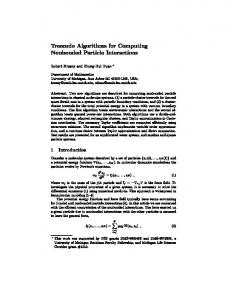
Fig. 2. Segments in proof of Lemma 6.

4

Improved Algorithms

Our techniques are built upon the use of decreasingly right-skew partitions, as reviewed in Section 3. Our improvements are based upon the following observation. An exact good partner for an index i need not be found if it can be determined that such a partner would result in density no greater than that of a segment already considered. This observation allows us to use a sweepline technique to replace the O(log L)-time binary searches used by Lin, Jiang and Chao [LJC02] with sequential searches that run with an amortized time of O(1). In particular, we make use of the following key lemma. Lemma 6 For a given j, assume A(j, j ′ ) is a maximum-density segment of those starting with index j, having L ≤ w(j, j ′ ) ≤ U, and ending with index in a given range [x, y]. For a given i < j, assume A(i, i′ ) is a maximum-density segment of those starting with index i, having L ≤ w(i, i′ ) ≤ U and ending in range [x, y]. If i′ > j ′ , then µ(j, j ′ ) ≥ µ(i, i′ ).

PROOF. A typical such configuration is shown in Figure 2. By assumption, both indices i′ and j ′ lie within the range [x, y]. Since L ≤ w(j, j ′ ) < w(j, i′ ) < w(i, i′ ) ≤ U, the optimality of A(j, j ′ ) guarantees that µ(j, j ′ ) ≥ µ(j, i′ ). This implies that µ(j, j ′ ) ≥ µ(j, i′ ) ≥ µ(j ′ + 1, i′ ). Since L ≤ w(j, j ′ ) < w(i, j ′) < w(i, i′ ) ≤ U, the optimality of A(i, i′ ) guarantees that µ(i, i′ ) ≥ µ(i, j ′ ), which in turn implies µ(j ′ + 1, i′ ) ≥ µ(i, i′ ) ≥ µ(i, j ′ ). Combining these inequalities, µ(j, j ′ ) ≥ µ(j, i′ ) ≥ µ(j ′ +1, i′ ) ≥ µ(i, i′ ), thus proving the claim that µ(j, j ′ ) ≥ µ(i, i′ ). 2

Our high level approach is thus to find good partners for each left endpoint i, considering those indices in decreasing order. However, rather than finding the true good partner for each i, our algorithm considers only matching indices which are less than or equal to all previously found good partners, in accordance with Lemma 6. In this way, as we sweep from right to left over the left endpoints i, we also sweep from right to left over the relevant matching indices. 7

4.1 Maximum-Density Segment with Width at Least L

In this section, we consider the problem of finding a segment with the maximum possible density among those of width at least L. We begin by introducing a sweep-line data structure which helps manage the search for good partners.

4.1.1 A Sweep-Line Data Structure The data structure developed in this section is designed to answer queries of the following type for a given range [x, y], specified upon initialization. For left index i, the goal is to return a matching right index i′ such that µ(i, i′ ) is maximized, subject to the constraints that i′ ∈ [x, y] and that w(i, i′ ) ≥ L. No upper bound on the segment length is considered by this structure. In order to achieve improved efficiency, the searches are limited in the following two ways: (1) The structure can be used to find matches for many different left indices, however such queries must be made in decreasing order. (2) When asked to find the match for a left index, the structure only finds the true good partner in the case that the good partner has index less than or equal to all previously returned indices. Our data structure augments the right-skew pointers for a given interval with additional information used to speed up searches for good partners. The structure contains the following state information, relative to given parameters 1 ≤ x ≤ y ≤ n: • A (static) array, p[k] for x + 1 ≤ k ≤ y, where A(k, p[k]) is the leftmost segment of DRSP(A(k, y)). • A (static) sorted list, S[k], for each x + 1 ≤ k ≤ y, containing all indices j for which p[j] = k. • Two indices ℓ and u (for “lower” and “upper”), whose values are nonincreasing as the algorithm progresses. • A variable, b (for “bridge”), which is maintained so that A(b, p[b]) is the segment of DRSP(A(ℓ, y)) which contains index u. These data structures are initialized with procedure InitializeL(x, y), given in Figure 3. An example of an initialized structure is given in Figure 4. Lines 1– 8 of InitializeL set the values p[k] as was done in the algorithm of Lin, Jiang and Chao [LJC02]. Therefore, we state the following fact, proven in that preceding paper.

8

1 2 3 4 5 6 7 8 9

procedure InitializeL(x, y) assumes 1 ≤ x ≤ y ≤ n for i ← y downto x + 1 do S[i] ← ∅ p[i] ← i while ((p[i] < y) and (µ(i, p[i]) ≤ µ(p[i] + 1, p[p[i] + 1]))) do p[i] ← p[p[i] + 1] end while Insert i at beginning of S[p[i]] end for ℓ ← y; u ← y; b ← y Fig. 3. InitializeL operation.

ai p[i] S[i]

1

2

3

4

5

6

7

8

9 10 11 12 13 14

1

4

1

5

4

5

4

3

4

2

7

4

6

6

7

9

9 14 11 13 13 14

5

3

8

6

7

9

2

4

1

4

11

2

5

3

12 10 13 14

Fig. 4. Example of data structure after InitializeL(1, 14), with wi = 1 for all i.

Lemma 7 After a call to InitializeL(x, y), p[k] is set for all x + 1 ≤ k ≤ y such that A(k, p[k]) is the leftmost segment of DRSP(A(k, y)). We also prove the following nesting property of decreasingly right-skew partitions. Lemma 8 Consider two segments A(x1 , y) and A(x2 , y) with a common right endpoint. Let A(k, k ′ ) be a segment of DRSP(A(x1 , y)) and let A(m, m′ ) be a segment of DRSP(A(x2 , y)). It cannot be the case that k < m ≤ k ′ < m′ .

PROOF. If A(k, k ′ ) is a segment of DRSP(A(x1 , y)), a repeated application of Lemma 2 assures that A(k, k ′ ) is the leftmost segment of DRSP(A(k, y)) and that A(k, k ′ ) is the longest possible right-skew segment of those starting with index k. We assume for contradiction that k < m ≤ k ′ < m′ , and consider the following three non-empty segments, A(k, m − 1), A(m, k ′ ) and A(k ′ + 1, m′ ). Since A(k, k ′ ) is right-skew, it must be that µ(k, m − 1) ≤ µ(m, k ′ ). Since A(m, m′ ) is right-skew, it must be that µ(m, k ′ ) ≤ µ(k ′ + 1, m′ ). In this case, it must be that the combined segment A(k, m′ ) is right-skew (this fact can be explicitly proven by application of Lin, Jiang and Chao’s Lemma 4 [LJC02]). Therefore 9

1 2 3 4 5 6 7 8 9 10 11 12 13

procedure FindMatchL(i) while (ℓ > 1 + max(x, Li )) do ℓ← ℓ−1 if (p[ℓ] ≥ u) then b←ℓ end if end while while (u ≥ ℓ) and (µ(i, b − 1) > µ(i, p[b])) do u←b−1 if (u ≥ ℓ) then b ← minimum k ∈ S[u] such that k ≥ ℓ end if end while return u

// decrease ℓ

// bitonic search

Fig. 5. FindMatchL(i) operation.

the existence of right-skew segment A(k, m′ ) contradicts the assumption that A(k, k ′ ) is the longest right-skew segment beginning with index k. 2 Corollary 9 There cannot exist indices k and m such that k < m ≤ p[k] < p[m].

PROOF. A direct result of Lemmas 7–8. 2

We introduce the main query routine, FindMatchL, given in Figure 5. Lemma 10 If b is the minimum value satisfying ℓ ≤ b ≤ u ≤ p[b], then A(b, p[b]) is the segment of DRSP(A(ℓ, y)) which contains index u.

PROOF. By Lemma 7, A(b, p[b]) is the leftmost segment of DRSP(A(b, y)), and as b ≤ u ≤ p[b], A(p, p[b]) contains index u. By repeated application of Lemma 2, DRSP(A(ℓ, y)) equals A(ℓ, p[ℓ]), A(p[ℓ] + 1, p[p[ℓ] + 1]), and so on, until reaching right endpoint y. We claim that A(b, p[b]) must be part of that partition. If not, there must be some other A(m, p[m]) with m < b ≤ p[m]. By Lemma 8, it must be that p[m] ≥ p[b], yet then we have m < b ≤ u ≤ p[b] ≤ p[m]. Such an m violates the assumed minimality of b. 2 Lemma 11 Whenever line 7 of FindMatchL() is evaluated, b is the minimum value satisfying ℓ ≤ b ≤ u ≤ p[b], if such a value exists. 10

PROOF. We show this by induction over time. When initialized, ℓ = b = u = p[b] = y, and thus b is the only satisfying value. The only time this invariant can be broken is when the value of ℓ or u changes. ℓ is changed only when decremented at line 2 of FindMatchL. The only possible violation of the invariant would be if the new index ℓ satisfies ℓ ≤ u ≤ p[ℓ]. This is exactly the condition handled by lines 3–4. Secondly, u is modified only at line 8 of FindMatchL. Immediately before this line is executed the invariant holds. At this point, we claim that p[k] ≤ b − 1 for any values of k such that ℓ ≤ k < b. For k < b, Corollary 9 implies that either p[k] < b or p[k] ≥ p[b]. If it were the case that p[k] ≥ p[b] ≥ u this would violate the minimality of b assumed at line 7. Therefore, it must be that p[k] ≤ b − 1 for all ℓ ≤ k ≤ b − 1. As u is reset to b − 1, the only possible values for the new bridge b are those indices k with p[k] = u, which is precisely the set S[b − 1] considered at line 10 of FindMatchL. 2 Lemma 12 Assume FindMatchL(i) is called with a value i less than that of all previous invocations and such that Li < y. Let m0 be the most recently returned value from FindMatchL() or y if this is the first such call. Let A(i, m) be a maximum-density segment of those starting with i, having width at least L, and ending with m ∈ [x, y]. Then FindMatchL(i) returns the value min(m, m0 ). PROOF. All segments which start with i, having width at least L and ending with m ∈ [x, y] must include interval A(i, max(x, Li )). The loop starting at line 1 ensures that variable ℓ = 1 + max(x, Li ) upon the loop’s exit. As discussed in Section 3, the optimal such m must either be ℓ − 1 or else among the right endpoints of DRSP(A(ℓ, y)). Since u is only set within FindMatchL, it must be that u = m0 upon entering the procedure. By Lemmas 10–11, A(b, p[b]) is the right-skew segment containing index u in DRSP(A(ℓ, y)). If µ(i, b − 1) ≤ µ(i, p[b]), the good partner must have index at least p[b] ≥ u, by Lemma 4. In this case, the while loop is never entered, and the procedure returns m0 = min(m, m0 ). In any other case, the true good partner for i is less than or equal to m0 , and this good partner is found by the while loop of line 1, in accordance with Lemmas 3–4. 2 Lemma 13 If FindMatchL(i) returns value i′ , it must be the case that for some j ≥ i, segment A(j, i′ ) is a maximum-density segment of those starting with j, having width at least L, and ending in [x, y]. PROOF. We prove this by induction over the number of previous calls to FindMatchL. i′ = m, as defined in the statement of Lemma 12, then this claim 11

is trivially true for j = i. Otherwise, i′ is equal to the same value returned by the previous call to FindMatchL, and by induction, there is some j ≥ i such that segment A(j, i′ ) is such a maximum-density segment. 2 Lemma 14 The data structure supports its operations with amortized running times of O(y − x + 1) for InitializeL(x, y), and O(1) for FindMatchL(i). PROOF. With the exception of lines 2, 7 and 9, the initialization procedure is simply a restatement of the algorithm given by Lin, Jiang and Chao [LJC02] for constructing the right-skew pointers. An O(y−x+1)-time worst-case bound was proven by those authors. In analyzing the cost of FindMatchL we note that variables ℓ and u are initialized to value y at line 9 of InitializeL. Variable ℓ is modified only when decremented at line 2 of FindMatchL and remains at least x + 1 due to the condition at line 1. Therefore, the loop of lines 1–6 executes at most y − x + 1 times and this cost can be amortized against the initialization cost. Variable u is modified only at line 8. By Lemma 11, x < ℓ ≤ b ≤ u ≤ p[b], and so this line results in a strict decrease in the value of u yet u remains at least x. Therefore, the while loop of lines 7–12 executes O(y − x + 1) times. The only step within that loop which cannot be bounded by O(1) in the worst case is that of line 10. However, since each k appears in list S[u] for a distinct value of u, the overall cost associated with line 10 is bounded by O(y − x + 1). Therefore the cost of this while loop can be amortized as well against the initializaiton cost. An O(1) amortized cost per call can account for all remaining instructions outside of the loops. 2 4.1.2 An O(n)-time Algorithm In Figure 6, we present a linear-time algorithm for the maximum-density segment problem subject only to a lower bound of L on the segment width. The algorithm makes use of the data structure developed in Section 4.1.1. Theorem 15 Given a sequence A, the algorithm MaximumDensitySegmentL finds the maximum-density segment of those with width at least L. PROOF. To prove the correctness, assume that µ ˆ is the density of an optimal such segment. First, we note that for any value i, Lemma 12 assures that g[i] is set such that g[i] ≥ Li . Therefore, µ(k, g[k]) ≤ µ ˆ for all k for which g[k] was defined. We claim that for some k, value g[k] is set such that µ(k, g[k]) ≥ µ ˆ. Assume ′ that the maximum density µ ˆ is achieved by some segment A(i, i ). Since it 12

1 2 3 4 5 6 7 8 9 10 11

procedure MaximumDensitySegmentL(A, L) [calculate partial sums, Li , as discussed in Section 2] call InitializeL(1, n) to create data stucture i0 ← maximum index such that Li0 is well-defined for i ← i0 downto 1 do if (Li = y) then // only one feasible right index g[i] ← y else g[i] ← FindMatchL(i) end if end for return (k, g[k]) which maximizes µ(k, g[k]) for 1 ≤ k ≤ i0

Fig. 6. Algorithm for finding maximum-density segment with width at least L

must be that Li is well-defined, we consider the pass of the loop starting at line 4 for such an i. Lemma 13 assures us that if FindMatchL is called, it either returns i′ or else it must be the case that for some j > i, g[j] < i′ In this case, as U is unbounded, Lemma 6 assures us that µ(j, g[j]) ≥ µ(i, i′ ) = µ ˆ. And thus MaximumDensitySegmentL returns a segment with density µ ˆ. 2 Theorem 16 Given a sequence A of length n, MaximumDensitySegmentL runs in O(n) time.

PROOF. This is a direct consequence of Lemma 14. 2

4.2 Maximum-Density Segment with Width at Least L and at Most U In this section, we consider the problem of finding a segment with the maximum possible density among those of width at least L and at most U. At first glance, the sweeping of variable u in the previous algorithm appears similar to placing an explicit upper bound on the width of the segments of interest for a given left index i. In locating the good partner for i, a sequential search is performed over right-skew segments of DRSP(A(Li + 1, n)). The repeated decision of whether it is advantageous to include the bridge segment A(b, p[b]) is determined in accordance with the bitonic property of Lemma 4. The reason that this technique does not immediately apply to the case with an explicit upper bound of U is the following. If the right endpoint of the bridge, p[b], is strictly greater than Ui , considering the effect of including the entire bridge may not be relevant. To properly apply Lemmas 3–4, we must consider segments of DRSP(A(Li + 1, Ui )) as opposed to DRSP(A(Li + 1, n)). 13

1 2 3 4 5 6 7

procedure InitializeU(x, y) assumes 1 ≤ x ≤ y ≤ n for i ← x + 1 to y do q[i] ← i while ((q[i] > x) and (µ(q[q[i] − 1], q[i] − 1) ≤ µ(q[i], i))) do q[i] ← q[q[i] − 1] end while end for u←y Fig. 7. InitializeU operation.

ai q[i]

1

2

3

4

5

6

7

8

9 10 11 12 13 14

1

4

1

5

4

5

4

3

4

2

3

3

3

3

3

8

8 10 10 12 10 10

1

4

2

5

3

Fig. 8. Example of data structure after InitializeU(1, 14), with wi = 1 for all i.

4.2.1 Another Sweep-Line Data Structure Recall that the structure of Section 4.1.1 focused on finding segments beginning with i, ending in [x, y] and subject to a lower bound on the resulting segment width. Therefore, as i was decreased, the effective lower bound, Li , on the matching endpoint can only decrease. The decomposition of interest was DRSP(A(Li , y)), and such decompositions were simultaneously represented for all possible values of Li by the right-skew pointers, p[k]. In this section, we develop another sweep-line data structure that we used to locate segments beginning with i, ending in [x, y] and subject to an upper bound on the resulting segment width (but with no explicit lower bound). For a given i, the decomposition of interest is DRSP(A(x + 1, Ui )). However, since Ui decreases with i, our new structure is based on representing the decreasingly right-skew partitions for all prefixes of A(x + 1, y), rather than all suffixes. We assign values q[k] for x + 1 ≤ k ≤ y such that A(q[k], k) is the rightmost segment of DRSP(A(x + 1, k)). Though there are clear symmetries between this section and Section 4.1.1, there is not a perfect symmetry; in fact the structure introduced in this section is considerably simpler. The lack of perfect symmetry is because the concept of right-skew segments, used in both sections, is oriented. The initialization routine for this new structure is presented in Figure 7. An example of an initialized structure is given in Figure 8. The redesign of the initialization routine relies on a simple duality when compared with the corresponding routine of Section 4.1.1. One can easily verify that an execution of this routine on a segment A(x, y) sets the values of array q precisely as 14

1 2 3 4 5 6 7

procedure FindMatchU(i) while (u > Ui ) do u←u−1 end while while (u > x) and (µ(i, q[u] − 1) > µ(i, u)) do u ← q[u] − 1 end while return u

// decrease u

// bitonic search

Fig. 9. FindMatchU(i) operation.

the original version would set the values of array p if run on a reversed and negated copy of A(x, y). Based on this relationship, we claim the following dual of Lemma 7 without further proof. Lemma 17 Immediately after InitializeU(x, y), the segment A(q[k], k) is the rightmost segment of DRSP(A(x + 1, k)), for all k in the range [x + 1, y]. We now present the main query routine, FindMatchU, given in Figure 9, and discuss its behavior. Lemma 18 Assume FindMatchU(i) is called with a value i less than that of all previous invocations and such that x ≤ Ui ≤ y. Let m0 be the most recently returned value from FindMatchU() or y if this is the first such call. Let A(i, m) be a maximum-density segment of those starting with i, having width at most U, and ending with m ∈ [x, m0 ]. Then FindMatchU(i) returns the value m.

PROOF. Combining the constraints that w(i, m) ≤ U and that m ∈ [x, m0 ], it must be that m ≤ min(Ui , m0 ). When entering the procedure, the variable u has value m0 . The loop starting at line 1 ensures that variable u = min(Ui , m0 ) upon the loop’s exit. The discussion in Section 3 assures us that the optimal m ∈ [x, u] must either be x or else among the right endpoints of DRSP(A(x + 1, u)). Based on Lemma 17, A(q[u], u) is the rightmost segment of DRSP(A(x + 1, u)) and so the loop condition at line 4 of FindMatchU is a direct application of Lemma 4. 2 Lemma 19 The data structure supports its operations with amortized running times of O(y − x + 1) for InitializeU(x, y), and O(1) for FindMatchU(i), so long as Ui ≥ x for all i.

PROOF. The initialization procedure has an O(y − x + 1)-time worst-case bound, as was the case for the similar routine in Section 4.1.1. 15

To account for the cost of FindMatchU, we note that u is initialized to value y at line 7 of InitializeU. It is only modified by lines 2 and 5 of the routine, and we claim that both lines strictly decrease the value. This is obvious for line 2, and for line 5, it follows for FindMatchU, since q[u] ≤ u in accordance with Lemma 17. We also claim that u is never set less than x. Within the loop of lines 1–3, this is due to the assumption that Ui ≥ x. For the loop of lines 4– 7, it is true because q[u] ≥ x + 1 in accordance with Lemma 17. Therefore, these loops execute at most O(y − x + 1) times combined and this cost can be amortized against the initialization cost. An O(1) amortized cost per call can account for checking the initial test condition before entering either loop. 2

4.2.2 An O(n)-time Algorithm for the Uniform Model In this section, we present a linear-time algorithm for the uniform maximumdensity segment problem subject to both a lower bound L and an upper bound U on the segment width, with L < U. Our strategy is as follows. We pre-process the original sequence by breaking it into blocks of cardinality exactly U − L (except, possibly for the last block). For each such block, we maintain two sweep-line data structures, one as in Section 4.1.1 and one as in Section 4.2.1. For a given left index i, a valid good partner must lie in the range [Li , Ui ]. Because we consider the uniform model, such an interval had cardinality precisely (U − L + 1) and thus overlaps exactly two of the pre-processed blocks. For α = (U − L)⌈Li /(U − L)⌉, we search for a potential partner in the range [Li , α] using the data structure of Section 4.1.1, and for a potential partner in the range [α + 1, Ui ] using the data structure of Section 4.2.1. Though we are not assured of finding the true good partner for each i, we again find the global optimum, in accordance with Lemma 6. Our complete algorithm is given in Figure 10. Theorem 20 Given a sequence A of length n for which wi = 1 for all i, and parameters L < U, the algorithm MaximumDensitySegmentLU finds the maximum-density segment of those with width at least L and at most U.

PROOF. Because wi = 1 for all i, the interval [Li , Ui ] has cardinality precisely (U − L + 1). We note that z is chosen at line 12 so that Li lies within BlockL [z] and that Ui lies within BlockU [z + 1]. To prove the correctness, assume that µ ˆ is the density of an optimal such segment. First, we claim that L ≤ w(i, g[i]) ≤ U for any i and thus that the algorithm cannot possibly return a density greater than µ ˆ. This is a direct 16

1 2 3 4 5 6 7 8 9 10 11 12 13 14 15 16 17 18 19 20 21

procedure MaximumDensitySegmentLU(A, L, U ) [calculate values Li and Ui , as discussed in Section 2] lef tend ← 1 while (lef tend < n) do // initialize blocks rightend ← min(n, lef tend + (U − L) − 1) z ← (lef tend − 1)/(U − L) BlockL [z] ← InitializeL(lef tend, rightend) BlockU [z] ← InitializeU(lef tend, rightend) lef tend ← lef tend + (U − L) end while i0 ← maximum index such that Li0 is well-defined for i ← i0 downto 1 do z ← ⌈Li /(U − L)⌉ // determine which blocks to search gL [i] ← FindMatchL(i) for BlockL [z] gU [i] ← FindMatchU(i) for BlockU [z + 1] if (µ(i, gL[i]) ≥ µ(i, gU [i])) then g[i] ← gL [i] else g[i] ← gU [i] end if end for return (k, g[k]) which maximizes µ(k, g[k]) for 1 ≤ k ≤ i0

Fig. 10. Algorithm for finding maximum-density segment with width at least L and at most U

result of Lemma 12 in regard to the block searched at line 13 and Lemma 18 in regard to the block searched at line 14. We then claim that for some k, value g[k] is set such that µ(k, g[k]) ≥ µ ˆ. Assume that the maximum density µ ˆ is achieved by some segment A(i, i′ ). Since it must be that Li is well-defined, we consider the pass of the loop starting at line 11 for such an i. We show that either g[i] = i′ or else there exists some j > i such that µ(j, g[j]) ≥ µ(i, i′ ). If i′ lies within BlockL [z] then we apply the same reasoning about the call to FindMatchL at line 13, as we did in the proof of Theorem 15. If i′ lies within BlockU [z + 1] then we consider the behavior of the call to FindMatchU(i) at line 14. If that call does not return i′ then it must be that i′ > m0 as defined in Lemma 18. Since the return values of this method are non-increasing, we let j be the largest index for which the returned g[j] < i′ . At the onset of that call to FindMatchU it must have been that m0 ≥ i′ and therefore we can apply Lemma 6 to deduce that µ(j, g[j]) ≥ µ(i, i′ ). Thus MaximumDensitySegmentLU returns a segment with density µ ˆ. 2 Theorem 21 Given a sequence A of length n for which wi = 1 for all i, the 17

algorithm MaximumDensitySegmentLU runs in O(n) time.

PROOF. This is a consequence of Lemmas 14 and 19. The calls to the initialization routines in the loop of lines 3–9 runs in O(n) time, as each initialization routine is called for a set of blocks which partition the original sequence. Similarly, the cost of all the calls to FindMatchL and FindMatchU in the loop of lines 11–20 can be amortized against the corresponding initializations. 2

4.2.3 An O(n + n log(U − L + 1))-time Algorithm for a More General Model With general values of wi , the algorithm in Section 4.2.2 is insufficient for one of two reasons. If values of wi > 1 are allowed, it may be that an entire interval [Li , Ui ] falls in a single block, in which case neither of the sweep-line data structures suffice. Alternatively, if values of wi < 1 are allowed, then an interval [Li , Ui ] might span an arbitrary number of blocks. Always searching all such blocks might result in ω(n) overall calls to FindMatchL or FindMatchU. In this section, we partially address the general case, providing an O(n + n log(U − L + 1))-time algorithm when wi ≥ 1 for all i. This condition assures us that the interval [Li , Ui ] has cardinality at most (U − L + 1). Rather than rely on a single partition of the original sequence into fixed-sized blocks, we will create O(log(U − L + 1)) partitions, each of which uses fixed-sized blocks, for varying sizes. Then we show that the interval [Li , Ui ] can be covered with a collection of smaller blocks in which we can search. For ease of notation, we assume, without loss of generality, that the overall sequence A is padded with values so that it has length n which is a power of two. We consider n blocks of size 1, n/2 blocks of size 2, n/4 blocks of size 4, and so on until n/2β blocks of size 2β , where β = ⌊log2 (U − L + 1)⌋. Specifically, we define block Bj,k = A(1 + j ∗ 2k , (j + 1) ∗ 2k ) for all 0 ≤ k ≤ β and 0 ≤ j < n/2k . We begin with the following lemma. Lemma 22 For any interval A(p, q) with cardinality at most U − L + 1, we can compute, in O(1 + β) time, a collection of O(1 + β) disjoint blocks such that A(p, q) equals the union of the blocks. The algorithm CollectBlocks is given in Figure 11, and a sample result is shown in Figure 12. It is not difficult to verify the claim. Theorem 23 Given a sequence A of length n for which wi ≥ 1 for all i, a maximum-density segment of those with width at least L and at most U can be found in O(n + n log(U − L + 1)) time. 18

1 2 3 4 5 6 7 8 9 10 11 12 13 14 15 16 17

procedure CollectBlocks(p, q) s ← p; k ← 0; while (2k + s − 1 ≤ q) do while (2k+1 + s − 1 ≤ q) do k ←k+1 end while j ← ⌈s/2k ⌉ − 1 Add block Bj,k to the collection k ←k+1 end while while (s ≤ q) do while (2k + s − 1 > q) do k ←k−1 end while j ← ⌈s/2k ⌉ − 1 Add block Bj,k to the collection k ←k−1 end while Fig. 11. Algorithm for finding collection of blocks to cover an interval

Fig. 12. A collection of blocks for a given interval

PROOF. The algorithm is given in Figure 13. First, we discuss the correctness. Assume that the global maximum is achieved by A(i, i′ ). We must simply show that this pair, or one with equal density, was considered at line 14. By Lemma 22, i′ must lie in some Bj,k returned by CollectBlocks(Li , Ui ). Because µ(i, i′ ) is a global maximum, the combination of Lemmas 6 and 12 assures us that FindMatchL() at line 10 will return i′ or else some earlier pair which was found has density at least as great. We conclude by showing that the running time is O(n + nβ). Notice that for a fixed k, blocks Bj,k for 0 ≤ j < n/2k − 1 comprise a partition of the original input A, and thus the sum of their cardinalities is O(n). Thefefore, for a fixed k, lines 4–6 run in O(n) time by Lemma 14, and overall lines 3–7 run in O(nβ) time. Each call to CollectBlocks from line 9 runs in O(1 + β) time by Lemma 22, and produces O(1 + β) blocks. Therefore, the body of that loop, lines 9–14, executes O(n + nβ) times over the course of the entire algorithm. 19

1 2 3 4 5 6 7 8 9 10 11 12 13 14 15

procedure MaximumDensitySegmentLU2(A, L, U) [calculate values Li and Ui , as discussed in Section 2] β ← ⌊log2 (U − L + 1)⌋; µmax ← −∞; for k ← 0 to β do for j ← 0 to n/2k − 1 do Bj,k ← InitializeL(1 + j ∗ 2k , (j + 1) ∗ 2k ) end for end for i0 ← maximum index such that Li is defined foreach Bj,k in CollectBlocks(Li , Ui ) do temp ← FindMatchL(i) if µ(i, temp) > µmax then µmax ← µ(i, temp); record endpoints (i, temp) end if end foreach end for

Fig. 13. Algorithm for maximum-density segment with width at least L, at most U

Finally, we must account for the time spent in all calls to FindMatchL from line 10. Rather than analyze these costs chronologically, we account for these calls by considering each block Bj,k over the course of the algorithm. By Lemma 14, each of these calls has an amortized cost of O(1), where that cost is amortized over the initialization cost for that block. 2

Acknowledgments We wish to thank Yaw-Ling Lin for helpful discussions.

References [AS98]

N. N. Alexandrov and V. V. Solovyev. Statistical significance of ungapped sequence alignments. In Proceedings of Pacific Symposium on Biocomputing, volume 3, pages 461–470, 1998.

[Bar00]

G. Barhardi. Isochores and the evolutionary genomics of vertebrates. Gene, 241:3–17, 2000.

[BB86]

G. Bernardi and G. Bernardi. Compositional constraints and genome evolution. Journal of Molecular Evolution, 24:1–11, 1986.

20

[Ben86]

Jon Louis Bentley. Programming Pearls. Addison-Wesley, Reading, MA, 1986.

[Cha94]

B. Charlesworth. Genetic recombination: patterns in the genome. Current Biology, 4:182–184, 1994.

[DMG95]

L. Duret, D. Mouchiroud, and C. Gautier. Statistical analysis of vertebrate sequences reveals that long genes are scarce in GC-rich isochores. Journal of Molecular Evolution, 40:308–371, 1995.

[EW92]

Adam Eyre-Walker. Evidence that both G+C rich and G+C poor isochores are replicated early and late in the cell cycle. Nucleic Acids Research, 20:1497–1501, 1992.

[EW93]

Adam Eyre-Walker. Recombination and mammalian genome evolution. Proceedings of the Royal Society of London Series B, Biological Science, 252:237–243, 1993.

[FCC01]

Stephanie M. Fullerton, Antonio Bernardo Carvalho, and Andrew G. Clark. Local rates of recombination are positively corelated with GC content in the human genome. Molecular Biology and Evolution, 18(6):1139–1142, 2001.

[Fil87]

J. Filipski. Correlation between molecular clock ticking, codon usage fidelity of DNA repair, chromosome banding and chromatin compactness in germline cells. FEBS Letters, 217:184–186, 1987.

[FO99]

M. P. Francino and H. Ochman. Isochores result from mutation not selection. Nature, 400:30–31, 1999.

[FS90]

C. A. Fields and C. A. Soderlund. gm: a practical tool for automating DNA sequence analysis. Computer Applications in the Biosciences, 6:263–270, 1990.

[GGA+ 98] P. Guldberg, K. Gronbak, A. Aggerholm, A. Platz, P. thor Straten, V. Ahrenkiel, P. Hokland, and J. Zeuthen. Detection of mutations in GC-rich DNA by bisulphite denaturing gradient gel electrophoresis. Nucleic Acids Research, 26(6):1548–1549, 1998. [HDV+ 91] R. C. Hardison, D. Drane, C. Vandenbergh, J.-F. F. Cheng, J. Mansverger, J. Taddie, S. Schwartz, X. Huang, and W. Miller. Sequence and comparative analysis of the rabbit alpha-like globin gene cluster reveals a rapid mode of evolution in a G+C rich region of mammalian genomes. Journal of Molecular Biology, 222:233–249, 1991. [HHJ+ 97] W. Henke, K. Herdel, K. Jung, D. Schnorr, and S. A. Loening. Betaine improves the PCR amplification of GC-rich DNA sequences. Nucleic Acids Research, 25(19):3957–3958, 1997. [Hol92]

G. P. Holmquist. Chromosome bands, their chromatin flavors, and their functional features. American Journal of Human Genetics, 51:17–37, 1992.

21

[Hua94]

X. Huang. An algorithm for identifying regions of a DNA sequence that satisfy a content requirement. Computer Applications in the Biosciences, 10(3):219–225, 1994.

[IAY+ 96]

K. Ikehara, F. Amada, S. Yoshida, Y. Mikata, and A. Tanaka. A possible origin of newly-born bacterial genes: significance of GC-rich nonstop frame on antisense strand. Nucleic Acids Research, 24(21):4249–4255, 1996.

[Inm66]

R. B. Inman. A denaturation map of the 1 phage DNA molecule determined by electron microscopy. Journal of Molecular Biology, 18:464–476, 1966.

[JFN97]

Ruzhong Jin, Maria-Elena Fernandez-Beros, and Richard P. Novick. Why is the initiation nick site of an AT-rich rolling circle plasmid at the tip of a GC-rich cruciform? The EMBO Journal, 16(14):4456–4466, 1997.

[LJC02]

Y. L. Lin, T. Jiang, and K. M. Chao. Algorithms for locating the length-constrained heaviest segments, with applications to biomolecular sequence analysis. Journal of Computer and System Sciences, 2002. To appear.

[MHL01]

Shin-ichi Murata, Petr Herman, and Joseph R. Lakowicz. Texture analysis of fluorescence lifetime images of AT- and GC-rich regions in nuclei. Journal of Hystochemistry and Cytochemistry, 49:1443–1452, 2001.

[MRO97]

Cort S. Madsen, Christopher P. Regan, and Gary K. Owens. Interaction of CArG elements and a GC-rich repressor element in transcriptional regulation of the smooth muscle myosin heavy chain gene in vascular smooth muscle cells. Journal of Biological Chemistry, 272(47):29842– 29851, 1997.

[MTB76]

G. Macaya, J.-P. Thiery, and G. Bernardi. An approach to the organization of eukaryotic genomes at a macromolecular level. Journal of Molecular Biology, 108:237–254, 1976.

[NL00]

Anton Nekrutenko and Wen-Hsiung Li. Assessment of compositional heterogeneity within and between eukaryotic genomes. Genome Research, 10:1986–1995, 2000.

[RLB00]

P. Rice, I. Longden, and A. Bleasby. EMBOSS: The European molecular biology open software suite. Trends in Genetics, 16(6):276–277, June 2000.

[SA93]

L. Scotto and R. K. Assoian. A GC-rich domain with bifunctional effects on mRNA and protein levels: implications for control of transforming growth factor beta 1 expression. Molecular and Cellular Biology, 13(6):3588–3597, 1993.

22

[SAL+ 95] P. M. Sharp, M. Averof, A. T. Lloyd, G. Matassi, and J. F. Peden. DNA sequence evolution: the sounds of silence. Philosophical Transactions of the Royal Society of London Series B, Biological Sciences, 349:241–247, 1995. [Sel84]

Peter H. Sellers. Pattern recognition in genetic sequences by mismatch density. Bulletin of Mathematical Biology, 46(4):501–514, 1984.

[SFR+ 99] N. Stojanovic, L. Florea, C. Riemer, D. Gumucio, J. Slightom, M. Goodman, W. Miller, and R. Hardison. Comparison of five methods for finding conserved sequences in multiple alignments of gene regulatory regions. Nucleic Acids Research, 27:3899–3910, 1999. [SMRB83] P. Soriano, M. Meunier-Rotival, and G. Bernardi. The distribution of interspersed repeats is nonuniform and conserved in the mouse and human genomes. Proceedings of the National Academy of Sciences of the United States of America, 80:1816–1820, 1983. [Sue88]

N. Sueoka. Directional mutation pressure and neutral molecular evolution. Proceedings of the National Academy of Sciences of the United States of America, 80:1816–1820, 1988.

[WLOG02] Zhijie Wang, Eli Lazarov, Mike O’Donnel, and Myron F. Goodman. Resolving a fidelity paradox: Why Escherichia coli DNA polymerase II makes more base substitution errors in at- compared to GC-rich DNA. Journal of Biological Chemistry, 2002. To appear. [WSE+ 99] Y. Wu, R. P. Stulp, P. Elfferich, J. Osinga, C. H. Buys, and R. M. Hofstra. Improved mutation detection in GC-rich DNA fragments by combined DGGE and CDGE. Nucleic Acids Research, 27(15):e9, 1999. [WSL89]

K. H. Wolfe, P. M. Sharp, and Wen-Hsiung Li. Mutation rates differ among regions of the mammalian genome. Nature, 337:283–285, 1989.

[ZCB96]

S. Zoubak, O. Clay, and G. Bernardi. The gene distribution of the human genome. Gene, 174:95–102, 1996.

23