the lcp information from a text and its P os array, and present a linear-time algorithm for the problem ... Let Ai denote the suffix of A that starts at position i. ..... starting at l that consists of only rightmost edges, that is, viâ1 is the rightmost child of vi ...
Linear-Time Longest-Common-Prefix Computation in Suffix Arrays and Its Applications Toru Kasai1 , Gunho Lee2 , Hiroki Arimura1,3, Setsuo Arikawa1, and Kunsoo Park2? 1
3
Department of Informatics, Kyushu University Fukuoka 812-8581, Japan {arim,arikawa}@i.kyushu-u.ac.jp 2 School of Computer Science and Engineering Seoul National University, Seoul 151-742, Korea {ghlee,kpark}@theory.snu.ac.kr PRESTO, Japan Science and Technology Corporation, Japan
Abstract. We present a linear-time algorithm to compute the longest common prefix information in suffix arrays. As two applications of our algorithm, we show that our algorithm is crucial to the effective use of block-sorting compression, and we present a linear-time algorithm to simulate the bottom-up traversal of a suffix tree with a suffix array combined with the longest common prefix information.
1
Introduction
The suffix array [16] is a space-efficient data structure that allows efficient searching of a text for any given pattern. The suffix array is basically a sorted array P os of all the suffixes of a text. A suffix array for a text of length n can be built in O(n log n) time, and searching the text for a pattern of length m can be done in O(m log n) time by a binary search. When a suffix array is coupled with information about the longest common prefixes (lcps) of some elements in the suffix array, string searches can be speeded up to O(m + log n) time. The lcp information is usually computed during the construction of suffix arrays [15,11]. In some cases, however, the lcp information may not be readily available. In this paper we consider the lcp problem in suffix arrays that is to compute the lcp information from a text and its P os array, and present a linear-time algorithm for the problem. We also describe two applications of our algorithm, i.e., block-sorting compression and the substring traversal problem. The block-sorting algorithm [4] is a text compression method with good balance of compression ratio and speed. The original text can be decoded in linear time from block-sorting compression. An advantage of block-sorting compression is that the suffix array of the original text can also be obtained in the process of ?
This work was supported by the Brain Korea 21 Project.
A. Amir and G.M. Landau (Eds.): CPM 2001, LNCS 2089, pp. 181–192, 2001. c Springer-Verlag Berlin Heidelberg 2001
182
Toru Kasai et al. Text
Suffix tree
a
c a b b c a $
4 1
$ a
$ b c a $
c
b
b
8
c b c a $ 5
b b c a $ 2
9
a b b $ c a 6 $
$ 7 3
1 a
2 b
3 c
4 a
5 b
6 b
7 c
8 a
9 $
Suffix array 1 2 4 1
3 8
4 5
5 2
6 6
7 3
8 7
9 9
a $
b b c a $
b c a b b c a $
b c a $
c a b b c a $
c a $
$
a b b c a $
a b c a b b c a $
Fig. 1. An example of the suffix tree and the suffix array.
decoding. This means that we can compress a text and its suffix array together by simply using the block-sorting algorithm. This fact can be used for storing and transferring large full-text databases. However, the lcp information that is necessary for efficient searching is not obtained during the decoding of blocksorting compression. With our algorithm, block-sorting compression can be used more effectively to store a text and its suffix array. The substring traversal problem is to enumerate all branching substrings appearing in a given text. Although the problem is easily solvable by a bottom-up traversal of the suffix tree, recent large scale applications in bioinformatics and data mining require a more practical and scalable solution for the problem [2]. We present a simple linear-time algorithm that simulates the bottom-up traversal of a suffix tree with a suffix array combined with the lcp information. Our algorithm is space-efficient and I/O-efficient, i.e., it requires only 7n bytes including the text while the suffix tree requires at least 15n bytes, and it has a good I/O complexity of 5n/B blocks. Furthermore, the algorithm can be modified to solve a class of problems based on the occurrence count of each branching substring, which include the longest common substring problem [12], the square/tandem repeat problem [22], and the frequent/optimal substring problem [2,3,9]. Experiments on English text data show that our proposed algorithms run efficiently in practice.
2
Preliminaries
Let A = a1 a2 · · · an−1 $ be a text of length n ≥ 1. In what follows, we assume that A ends with a special end marker $ that does not appear in other positions. Let Ai denote the suffix of A that starts at position i. For a substring S of A, we denote by Occ(S, A) the set of all occurrences of S in A. Let ≡A be an equivalence relation on substrings defined as follows: For any substrings S, S 0 , the relation S ≡A S 0 holds if and only if Occ(S, A) = Occ(S 0 , A). A substring S of A is branching if S is the longest common prefix of distinct suffixes Ai and Aj (i 6= j).
Linear-Time Longest-Common-Prefix Computation
183
The suffix array of a text A [16] is a sorted array P os[1..n] of all the suffixes of A, i.e., P os[k] = i if Ai is lexicographically the k-th suffix. The suffix tree [17] is a data structure for storing all branching substrings of A, which is the compacted trie ST for all suffixes of A. The suffix tree has at most 2n − 1 nodes and can be stored in O(n) space. The suffix tree ST of a text of length n can be constructed in O(n) time [17,23,5]. The suffix array P os of A coincides with the list of the leaves of ST ordered from left to right. In Fig. 1, we show the suffix tree and the suffix array of string A = abcabbca$. We denote by str(v) the substring of A obtained by concatenating the labels on the path from the root to v. The following lemma is well known [17]. Lemma 1. Let S be any substring of A. Then, the following 1–3 are equivalent. 1. S is branching. 2. S is the unique longest member of the equivalence class of S w.r.t. ≡A . 3. S = str(v) for some internal node v of the suffix tree of A. We denote by lcp(A, B) the length of the longest common prefix between strings A and B. The lcps between suffixes that are adjacent in the sorted P os array are denoted by an array Height: Height[k] = lcp(Apos[k−1] , Apos[k] ) for 2 ≤ k ≤ n. All the necessary lcps for O(m + log n) search (called arrays Llcp and Rlcp in [16]) can be computed easily in O(n) time from array Height [11,15]. Therefore, we define the lcp problem as follows. Definition 1. The lcp problem in suffix arrays is to compute the Height array from a text A and its suffix array P os. For any substring S of A, the suffix array P os gives a compact representation of all occurrences of S. The set of all occurrences of S occupy a contiguous interval [L, R] ⊆ {1, . . . , n}, namely, Occ(S, A) = {P os[k] : L ≤ k ≤ R}. We call the pair (L, R) the rank interval of S. Then, the triple for S is the triple (L, R, H) of integers, where (L, R) is the rank interval of S and H = |S| is the length of S. If necessary, the substring can be immediately obtained by S = A[P os[L]..P os[L] + H − 1]. A bottom-up traversal of the suffix tree is any list L of its nodes such that each node appears exactly once in L, and a node appears in L only after all of its children appear. The post-order traversal [1] is an example of bottom-up traversals. A bottom-up substring traversal of A is a list L of the triples (L, R, H) for all branching substrings of A which is generated by a bottom-up traversal of the suffix tree of A. Then, the substring traversal problem is stated as follows. Definition 2. The substring traversal problem is to compute the substring traversal L for a text A. This problem is linear time solvable by a post-order traversal of the suffix tree ST . Unfortunately, it is difficult to solve this problem with the suffix array P os alone because P os has lost the information on tree topology. The array Height has the information on the tree topology which is lost in the suffix array P os.
184
Toru Kasai et al.
Fig. 2. An example of sorted suffixes and lcps.
Lemma 2. A substring S of a text A is branching if and only if there exists some rank 1 ≤ k ≤ n such that S is the longest common prefix of the adjacent suffixes AP os[k−1] and AP os[k] . From Lemma 2, we can compute the list of all branching substrings associated with the in-order traversal of ST simply by reporting A[P os[k]..P os[k] + Height[k] − 1] for every rank 1 ≤ k ≤ n. Unfortunately, the obtained list may contain duplicates since ST is not a binary tree. Furthermore, there is no obvious way to compute either the associated rank intervals (L, R) or the post-order traversal.
3
Linear-Time lcp Computation
In the lcp computation, we will use an intermediate array Rank. The array Rank is defined as the inverse function of P os, and it can be obtained immediately when the P os array is given: If P os[k] = i, then Rank[i] = k. 3.1
Properties of lcp
The lcp between two suffixes is the minimum of the lcps of all pairs of adjacent suffixes between them on the P os array [16]. That is, lcp(AP os[x] , AP os[z] ) = min {lcp(AP os[y−1] , AP os[y] )}. x 1, then Rank[P os[x − 1] + 1] < Rank[P os[x] + 1]. In this case, the lcp between AP os[x−1]+1 and AP os[x]+1 is one less than the lcp between AP os[x−1] and AP os[x] . Fact 3. If lcp(AP os[x−1] , AP os[x] ) > 1, then lcp(AP os[x−1]+1 , AP os[x]+1 ) = lcp(AP os[x−1] , AP os[x] ) − 1. Now we consider the following problem: compute the lcp between a suffix Ai and its adjacent suffix on P os when the lcp between Ai−1 and its adjacent suffix is known. For notational convenience, let p = Rank[i − 1] and q = Rank[i]. Also let j −1 = P os[p−1] and k = P os[q −1]. See Fig. 2. That is, we want to compute Height[q] when Height[p] is given. Lemma 3. If lcp(Aj−1 , Ai−1) > 1 then lcp(Ak , Ai ) ≥ lcp(Aj , Ai ). Proof. Since lcp(Aj−1 , Ai−1 ) > 1, we have Rank[j] < Rank[i] by Fact 2. Since Rank[j] ≤ Rank[k] = Rank[i] − 1, we get lcp(Ak , Ai ) ≥ lcp(Aj , Ai ) by Fact 1. Theorem 1. If Height[p] = lcp(Aj−1 , Ai−1 ) > 1 then Height[q] = lcp(Ak , Ai ) ≥ Height[p] − 1. Proof. lcp(Ak , Ai ) ≥ lcp(Aj , Ai ) = lcp(Aj−1 , Ai−1 ) − 1.
(by Lemma 3) (by Fact 3)
By Theorem 1, when the lcp between suffix Ai−1 and its adjacent suffix is h, suffix Ai and its adjacent suffix on P os has a common prefix of length at least h − 1. Therefore, it suffices to compare from the h-th characters for computing the lcp between suffix Ai and its adjacent suffix. If h is less than or equal to 1, we will compare from the first characters. 3.2
Algorithm and Analysis
We now present the algorithm GetHeight that solves the lcp problem in suffix arrays. By Theorem 1, we do not need to compare all characters when we compute the lcp between a suffix and its adjacent suffix on P os. To compute all the lcps of adjacent suffixes on P os efficiently, we examine the suffixes from A1 to An in order. Theorem 2. Algorithm GetHeight computes array Height in O(n).
186
Toru Kasai et al.
Algorithm GetHeight input: A text A and its suffix array Pos 1 for i:=1 to n do 2 Rank[Pos[i]] := i 3 od 4 h:=0 5 for i:=1 to n do 6 if Rank[i] > 1 then 7 k := Pos[Rank[i]-1] 8 while A[i+h] = A[j+h] do 9 h := h+1 10 od 11 Height[Rank[i]] := h 12 if h > 0 then h := h-1 fi 13 fi 14 od
Fig. 3. The linear-time algorithm for the lcp problem. Proof. The correctness of GetHeight follows from previous discussions. The execution time of the algorithm is proportional to the number of times line 9 is executed, since line 9 is the innermost loop of GetHeight. The value of h increases one by one in line 9, and it is always less than n due to the end marker $. Since the initial value of h is 0 and it decreases at most n times in line 12, h increases at most 2n times. Therefore, the time complexity of Algorithm GetHeight is O(n).
4 4.1
Application to Block-Sorting Compression Block-Sorting Compression
The block-sorting algorithm is a text compression method with good balance of compression ratio and speed [4,8]. It achieves speed comparable to dictionary compressors, but obtains compression close to the best statistical compressor. The block-sorting algorithm is used in bzip2 [21]. The encoder of block-sorting consists of three processes: the Burrows-Wheeler transformation, move-to-front encoding and entropy coding. The BurrowsWheeler transformation (BWT) is the most time-consuming process. It transforms a string A of length n by forming the n rotations (cyclic shifts) of A, sorting them lexicographically, and extracting the last character of each of the rotations. A string L is formed from these characters, where the i-th character of L is the last character of the i-th sorted rotation. In addition to L, the BWT computes the index I of the original string A in the sorted list of rotations. Fig. 4 is an example of BWT where A=’abraca’. A move-to-front encoding encodes an instance of a character ch by the count of distinct characters between itself and the previous occurrence of ch.
Linear-Time Longest-Common-Prefix Computation
187
Fig. 4. An example of the Burrows-Wheeler transformation.
As a result of BWT, the locality of characters of L goes higher than that of A [4]. So, when applied to the string L, the output of a move-to-front encoder will be dominated by low numbers, which can be effectively encoded with Huffman coding or run-length coding. The decoder of block-sorting is the reverse of the encoder. Decoding speed of an entropy code depends on the used method, but Huffman coding or run-length coding, which is generally used for encoding, can be reversed in linear time. A move-to-front code can be reversed in O(n) time, and the original string A, the reverse of the BWT, can be recovered from L and I in O(n) time. Therefore, the block-sorting decompression takes linear time in general. 4.2
Block-Sorting and Suffix Arrays
The first step of block-sorting, the BWT, is similar to the construction process of a suffix array. The BWT takes much time for sorting the suffixes. However, its reverse transformation from L and I to A is quickly computed in linear time by a radix-sort-like procedure. Moreover, the suffix array P os of A can be computed immediately when the compressed text is decoded. To search for a pattern using the suffix array more efficiently, the lcp information (Llcp and Rlcp) is required. The lcp information can be computed in O(n log n) time when the suffix array is constructed from the original text A. With our algorithm, the lcp information can be computed in O(n) time from the original text A and its P os array. Therefore, suffix arrays can be stored and used efficiently by the block-sorting compression. Since block-sorting has the effect of storing the compressed text and its suffix array, it can be used for storing and transferring large data. Sadakane and Imai presented a cooperative distributed text database management method unifying search and compression based on BWT [18]. Sadakane also presented a modified BWT for case-insensitive search with the suffix array [19]. Recently, Sadakane proposed a compressed text database system [20] based on the compressed suffix array [10]. Ferragina and Manzini [7,6] proposed a data structure that supports search operations without uncompressing the block-sorting compression.
188
Toru Kasai et al.
lca(lk-1 , lk)
root
Πk Πk-1
lk-1
lk
Fig. 5. An example of the rightmost branch decompositions.
5 5.1
Algorithm BottomUpTraverse; input: An ordered and compacted tree T with n ≥ 0 leaves `1 , . . . , `n . 1 S:={>} /* Initialize the stack S */ 2 for k:=1 to n+1 do /* k-th stage */ 3 v := lca(`k−1, `k ); 4 while (depth(top(S)) > depth(v)) do 5 v := Pop(S) and report v; od; 6 if (depth(top(S)) < depth(v)) then 7 Push(v, S); fi; 8 Push(`k, S); /* Set Sk = S */ 9 od /* for-loop */
Fig. 6. The algorithm to compute the postorder traversal of an ordered tree.
Bottom-Up Traversal of Suffix Trees Properties of the Post-Order Traversal
An ordered tree T is compacted if every internal node of T has at least two children. Let T be an ordered and compacted tree with n ≥ 0 leaves `1 , . . . , `n . In what follows, a path in T is always written in the upward direction. That is, a path (or upward path) is a sequence π = (v0 , v1 , . . . , vm ) (m ≥ 0) of nodes in T such that vi is the parent of vi−1 for every 1 ≤ i ≤ m. The length of π is |π| = m. A path π from the k-th leaf (1 ≤ k ≤ n) to the root is called the k-th branch of T and denoted by π(`k ). A node-depth of a node v, denoted by depth(v), is the length of the path from v to the root. We write u � v (u ≺ v) if a node u is an ancestor (proper ancestor) of node v. We denote by lca(u, v) the lowest common ancestor of nodes u and v and by π(`) the branch starting at a leaf `. Let ` be any leaf. A rightmost branch (RM branch, for short) starting with `, denoted by Π(`), is the longest branch π = (v0 = `, v1 , . . . , vm ) (m ≥ 0) starting at ` that consists of only rightmost edges, that is, vi−1 is the rightmost child of vi for every 1 ≤ i ≤ m. Π(`k ) is called the k-th RM branch. Since the set {Π(`1 ), . . . , Π(`n )} of all RM branches of T is called the RM branch decomposition of T since it is a partition of T . Fig. 5 shows an example of the RM branch decompositions, where each shadowed line indicates an RM branch (See below for the special node >). Lemma 4. The post-order traversal of an ordered tree T equals the concatenation Π(`1 ) · · · Π(`n ) of the RM branches of T from left to right.
5.2
Algorithm for Bottom-Up Substring Traversal
From now on, we consider a method to compute the post-order traversal of an ordered compacted tree T with n ≥ 0 leaves `1 , . . . , `n when the lowest common
Linear-Time Longest-Common-Prefix Computation
189
ancestors of adjacent leaves and the depth of a node are available. Fig. 6 shows the algorithm BottomUpTraverse for the problem. In the algorithm, we assume a special top node> such that > ≺ v for every v in T and special leaves `0 and `n+1 such that lca(`0 , `1 ) = lca(`n , `n+1 ) = > (See Fig. 5). Scanning the height array Height from left to right, the algorithm enumerates the nodes of T without duplicates by a sequence of push/pop operations to a stack S as follows. During the scan, a leaf node, say `k , is pushed into the stack S when it is first encountered at stage k and popped immediately at stage k + 1. The case for internal nodes is more complicated (See Fig. 5). Conceptually, a node v is pusded when it is visited from below at the first time and popped when it is visited at the last time in the depth-first search of T . An internal node v is pushed into the stack when the leftmost leaf of the second child of v, say `k , is encountered at the first time in the scan, i.e., v = lca(`k−1 , `k ). Then, v is popped from the stack S when the leftmost leaf of the next right sibling of v, is encountered in the scan. Then, p = lca(`k−1 , `k ) is the parent of v. Since the tree is compacted, the second leftmost leaf always exists for every internal node. Thus from Lemma 2, the algorithm BottomUpTraverse enumerates all nodes without duplicates by a scan of Height. To see that the algorithm correctly computes the post-order traversal of T , we need to know the precise contents of the stack during the scan. A key observation is that if an internal node v is lca(`k−1 , `k ) for some k then v is on the k-th branch from `k to the root and all nodes of Π(`k−1 ) are proper descendants of v. We gives the following lemma without proof due to the space limitation (See [14] for the complete proof). Lemma 5. Let us consider the algorithm BottomUpTraverse of Fig. 6. For any stage 1 ≤ k ≤ n + 1, the contents of the stack S at the beginning of the kth stage is the subsequence Sk = (vj0 , . . . , vjk ) of the k-th branch πk = (v0 = `k , v1 , . . . , vm = >) (m ≥ 0) such that for every 0 ≤ j ≤ m, vj ∈ Sk if and only if the following inclusion condition holds at position j: either (i) j = 0 or (ii) vj−1 is not the leftmost child of vj . From Lemma 5, we see that in the end of every stage k, the k-th RM branch Π(`k−1 ) is stored on the top of the stack S. Then, Π(`k−1 ) is deleted from the stack S when `k is encountered in the scan. By repeating this process, the algorithm finally outputs all RM branches Π(`1 ), . . . , Π(`n ) of T from left to right. Hence, the next lemma immediately follows from Lemma 4. Lemma 6. The algorithm BottomUpTraverse of Fig. 6 computes the post-order traversal of an ordered compacted tree with n leaves in O(n) time when the nodedepth for a node and the lowest common ancestor of adjacent leaves are constant time computable. Now we present a linear time algorithm for the substring traversal problem when the height array and the suffix array of A is given. Fig. 7 shows the algorithm TraverseWithArray to compute the list of triples for text A generated by the post-order traversal of a suffix tree. In the algorithm, we encode a node v
190
Toru Kasai et al.
Algorithm TraverseWithArray; input: The height array Height and the suffix array Pos for a text A; 1 S:= (-1, -1); n:=|T| /* Initialize the stack S */ 2 for k:=1 to n+1 do /* k-th stage */ 3 (Llca, Hlca) := (k-1, Height[k]); 4 (L, H) := top(S); 5 while (H > Hlca) do 6 (L, H) := pop(S), R := k-1; Then, report triple (L, R, H); 7 Llca := L; /* Update the left boundary */ 8 (L, H) := top(S); 9 od 10 if (H < Hlca) then 11 Push((Llca,Hlca), S); fi; 12 Push((k, n - Pos[k] + 1), S); /* Set Sk = S */ 13 od /* for-loop */
Fig. 7. A linear time algorithm for the substring traversal problem. by any pair (L, H) such that L and H are the any occurrence and the length of the substring str(v), respectively. The top node is encoded by (−1, −1). Recall that there were only two types of nodes processed in the algorithm BottomUpTraverse, a leaf and the lca of adjacent leaves. Thus for any rank 1 ≤ k ≤ n + 1, we encode v by (L, H) as follows: (i) if v is the leaf `k then (L, H) = (k, |AP os[k] |) = (k, n − P os[k] + 1) and (ii) if v is the lca node lca(`k−1 , `k ) then (L, H) = (k − 1, Height[k]). The depth of the node v is obviously given by H. From Lemma 6, we know that the algorithm correctly simulates ButtomUpTraverse. We then consider the computation of the rank intervals. Suppose a pair (L, H) is popped from the stack S at stage k and it represents a node v. By induction on the number of nodes below v on the (k − 1)-th path, we can show that L is the rank of the leftmost leaf of v, where the value of L is kept at the variable Llca at Line 7 of the algorithm. Since v is on the (k − 1)-th RM branch, R = k − 1 is obviously the rank of the rightmost leaf of v. Therefore, (L, R, H) is the triple of v, and the next theorem follows from Lemma 6. Theorem 3. The algorithm TraverseWithArray of Fig. 7 computes in O(n) time the list of all triples generated by the post-order traversal of the suffix tree of a text A of length n when the height array and the suffix array of A is given. Hence, the substring traversal problem is solvable in linear time when the height array Height of a text A is given. Since the algorithm TraverseWithArray makes only sequential I/Os and does not access the text A, we can also see that the algorithm is I/O efficient in the external I/O model of [24] (See [14]).
6
Experimental Results
We run experiments on a real dataset. For the height array construction, we implemented the naive O(n2 ) time algorithm (Abbreviated as NaiveHeight)
Linear-Time Longest-Common-Prefix Computation
191
and the linear time algorithm GetHeight (GetHeight). For the bottom-up substring traversal in Section 5, we implemented the algorithm with the suffix tree (TravTree), the naive algorithm with binary search on the suffix array (TravBinary), and the algorithm TraverseWithArray (TravHeight). Table 1. Comparison of the computation time on English texts. Height array construction Algorithm
NaiveHeight
GetHeight
Time (sec)
17.59
7.81
Substring traversal TravTree TravBinary TravHeight 2.07
13.62
1.94
In Table 1, we show the running time of the algorithms on an English text of 5.3MB [13] and a workstation (Sun UltraSPARC 300MHz, 256MB, g++ on Solaris 2.6). In the substring traversal, the preprocessing time for building the height array is not included. For the height array construction, we see from this table that GetHeight is faster than NaiveHeight more than twice on this test data. For the substring traversal, TravHeight is as fast as TravTree when the height array is precomputed, and faster than TravBinary even when the computation time of the height array is included.
References 1. A. V. Aho, J. E. Hopcroft and U. D. Ullman, Data Structures and Algorithms, Addison-Wesley, 1983. 2. H. Arimura, S. Arikawa and S. Shimozono, Efficient discovery of optimal wordassociation patterns in large text databases, New Generation Comput., 18, 49–60, 2000. 3. H. Arimura, H. Asaka, H. Sakamoto and S. Arikawa, Efficient discovery of proximity patterns with suffix arrays, In Proc. CPM 2001 , Poster paper, LNCS, SpringerVerlag, 2001. (In this volumn). 4. M. Burrows and D. J. Wheeler, A block-sorting lossless data compression algorithm, Digital Systems Research Center Research Report 124 , 1994. 5. M. Farach-Colton, P. Ferragina and S. Muthukrishnan, On the sorting-complexity of suffix tree construction, Journal of the ACM , Vol.47, No.6, 987–1011, 2000. 6. P. Ferragina and G. Manzini, Opportunistic data structures with applications, In Proc. 41st IEEE Symposium on Foundations of Computer Science, 390–398 2000. 7. P. Ferragina and G. Manzini, An experimental study of an opportunistic index, In Proc. 12th ACM-SIAM Symposium on Discrete Algorithms, 269–278 2001. 8. P. Fenwick, Block sorting text compression, In Proc. Australian Computer Science Communications, 18(1), 193–202, 1996. 9. R. Fujino, H. Arimura and S. Arikawa, Discovering unordered and ordered phrase association patterns for text mining, In Proc. PAKDD2000 , LNAI 1805, 281–293, 2000. 10. R. Grossi and J. S. Vitter, Compressed suffix arrays and suffix trees with applications to text indexing and string matching, In Proc. 32nd ACM Symposium on Theory of Computing, 397–406, 2000.
192
Toru Kasai et al.
11. D. Gusfield, An increment-by-one approach to suffix arrays and trees, Technical Report CSE-90-39 , UC Davis, Dept. Computer Science, 1990. 12. D. Gusfield, Algorithms on Strings, Trees, and Sequences: Computer Science and Computational Biology, Cambridge University Press, New York, 1997. 13. R. Harris, Abstract Index, Monash Univ (1998). 14. T. Kasai, H. Arimura and S. Arikawa, Efficient substring traversal with suffix arrays, DOI-TR 185, Feb. 2001. (First appeared as T. Kasai, Fast algorithms for the subword statistics problems with suffix arrays, Mc. Thesis, Dept. Informatics, Kyushu Univ.,1999, In Japanese.) 15. S. E. Lee and K. Park, A new algorithm for constructing suffix arrays, Journal of Korea Information Science Society (A), 24(7), 697–704, 1997. 16. U. Manber and G. Myers, Suffix arrays: A new method for on-line string searches, SIAM J. Computing, 22(5), 935–948 (1993). 17. E. M. McCreight, A space-economical suffix tree construction algorithm, Journal of the ACM, 23(2), 262–272, 1976. 18. K. Sadakane and H. Imai, A cooperative distributed text database management method unifying search and compression based on the Burrows-Wheeler transformation, In Proc. International Workshop on New Database Technologies for Collaborative Work Support and Spatio-Temporal Data Management , 434–445, 1998. 19. K. Sadakane, A modified Burrows-Wheeler transformation for case-insensitive search with application to suffix array compression, In Proc. Data Compression Conference, p.548, 1999. 20. K. Sadakane, Compressed text databases with efficient query algorithms based on the compressed suffix array, In Proc. 11th Annual International Symposium on Algorithms and Computation, 410–421, 2000. 21. J. Seward, http://sources.redhat.com/bzip2\/ 22. J. Stoye and D. Gusfield, Simple and flexible detection of contiguous repeats using a suffix tree, In Proc. CPM’98, LNCS, 140–152, 1998. 23. E. Ukkonen, On-line construction of suffix trees, Algorithmica 14, 249–260, 1995. 24. J. S. Vitter, External memory algorithms, In Proc. PODS’98 , 119–128 (1998).