Linear Time-Varying Models for Signal Processing P. van der Kloet and F.L. Neerhoff Delft University of Technology Faculty of Information Technology and Systems Electronics Research Laboratory Mekelweg 4, 2628 CD Delft, The Netherlands Phone: +31 (0)15 2787 353, Fax: +31 (0)15 2785 922 Email:
[email protected] Abstract— The solution of a linear time-invariant differential equation can be obtained as the output of a so-called canonical signal processing filter with the right hand side of the differential equation as input. Such a filter is build up with integrators, adders, multipliers and so on. One distinguishes in the literature between a series, a cascade and a parallel realization of the filter.The coefficients of the differential equation appear to be the multipliers in both, the series and parallel representation of the differential equation. The eigenvalues or poles of the differential equation are the multipliers in the cascade realization. On the basis of a number of recently obtained results one may expect that these three types of canonical representations also exist for linear time-varying differential equations. In this paper this problem is addressed. If we start with the series representation, then it is shown that the cascade realization uses the dynamic eigenvalues and that the parallel realization only in special cases equals the solution of the differential equation. Keywords— linear time-varying systems, canonical representations, dynamic eigenvalues.
I. Introduction The solution of a (higher order) linear timeinvariant scalar differential equation can be obtained as the output of a so-called canonical signal processing filter with the right-hand side of the differential equation as input. Generally, the analytical solution of this type of differential equations is obtained by solving a characteristic equation. With the solutions of this characteristic equation exponential functions are formed and any linear combination of these exponentials yield a solution of the homogeneous differential equation. Adding one particular solution of the inhomogeneous differential equation yields the general solution of the differential equation. This procedure fails when the coefficients of the differential equation become timedependent, so that we have a linear time-varying scalar differential equation. To overcome this difficulty, Zhu [1] started with the matrix state-space formulation for the differential
equation and derived a generalized eigenvalue problem. Earlier, this eigenvalue problem was already formulated by Wu [2]. Both did not obtain a full generalization of the classical theory for linear time-invariant differential equations. In the approach of Zhu it is quite complicated to solve the characteristic equations. Moreover, his state-space approach does not have completely arbitrarily matrices. In the state-space approach, there are two manners how to tackle the problem of solving a linear timevarying (matrix) differential equation. The first one exploits the shape of the solution as is done in the theory of linear time-invariant differential equations. This is essentially also followed by Zhu and Wu. The second approach first performs an operation on the complexity of the system matrix. One can try to perform operations such that the system matrix is reduced to a diagonal or a triangular matrix. These can be realized by applying a Riccati-Lyapunov transformation on the original differential equation. For triangularization the complete Riccati-Lyapunov transformation is the product of n−1 of such transformations. The i-th transformation is such that the elements left of the diagonal in the (n + 1 − i)-th row become zero. This procedure yields a modal expansion for the solution of the linear time-varying differential equation [3], [4]. These modes contain dynamic eigenvectors and dynamic eigenvalues as generalization of the classical algebraic eigenvectors and eigenvalues. The procedure followed to obtain these modal expansions needs in every step the solution of a set of differential equations of the Riccati type. Of course, the elements on the diagonal of the matrix transformed into a diagonal or triangular one represents the dynamic eigenvalues of the LTV system. The set of Riccati equations together with the equation for the dynamic eigenvalue on the diagonal can be combined into a set of equations which ressembles the characteristic equation. The reduction of this set of equations when we consider a linear time-invariant system in stead of a time-varying
436
system yields a set of Riccati equations which is indeed equivalent to the characteristic equation [5], [6], [7]. As a consequence, we see that the approach for linear time-varying differential equations yield solutions in the form of modal expansions. Each mode has a time-varying amplitude and in general a nonlinear phase. These reduce to the wellknown constant amplitude and linear phase for linear time-invariant differential equations. The same is true for characteristic equations. It is thus worth also for other properties of LTI systems to investigate their generalization to LTV sytems. In this paper canonical representations for signal processing [8], [9] are addressed. Our starting point is the differential equation dn x dn−1 x dx + a (t) + · · · + an−1 (t) + an (t)x = f (t) 1 n n−1 dt dt dt (1) This equivalent to the following system of first order equations x1 x1 0 . . . d .. . . (2) = A . + . f (t) dt xn−1 xn−1 0 xn xn 1 with
0 .. .
1
... .. . A= 0 0 ... −an (t) −an−1 (t) . . . and
£
x = 1 0 ...
0
1 −a1 (t)
The two other canonical representations for linear time-invariant systems, (the cascade and the parallel representation) will be generalized for linear timevarying systems. It will be shown that the cascade representation has the dynamic eigenvalues as multipliers (section II). The parallel representation is more cumbersome. This representation cannot be obtained in a straightforward manner. Therefore we will start in section III with a quite arbitrarily parallel realization and investigate the input-output relation. This will yield conditions for the multipliers in the cascade representation to give an equivalence between the series and the parallel representation (section III). Finally some conclusions will be formulated (section IV). II. The canonical cascade representation In order to derive the canonical cascade representation we introduce a second shorthand notation for (2) " # · ¸ " (1) # · ¸ d x1(1) I+ e 0 x1 n−1 n−1 = + f (t) (5) T −an−1 −a1 1 dt xn xn The meaning of the quantities introduced follows directly by comparison of (5) and (2), (3). Apply to (5) the transformation " # · ¸· ¸ (1) In−1 0 y1 x1 = T (6) pn−1 1 yn xn If p T is a solution of the Riccati differential equation
(3)
T T T T T T p˙ n−1 = −pn−1 I+ n−1 − pn−1 en−1 pn−1 − an−1 − a1 pn−1 (7) then
x1 ¤ . 0 .. xn
(4)
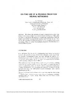
For this equation (1) or (2), (3), (4) we have a signal processing scheme as is depicted in figure 1. This figure shows the canonical series representation. f(t)
x(t)
T y˙ 1 = (I+ n−1 + en−1 pn−1 )y1 + en−1 yn
(8)
y˙ n = λn yn + f (t)
(9)
Moreover (4) and (6) show £ x = 1 0 ...
¤ 0 y1
(10)
If £ y1T = y1 . . .
¤ £ yn−1 , p1T = p1 . . .
pn−1
−an−2
−a n−1
−a n
(11)
then we can write (8) as y˙ 1 = Pn−1 y1 + en−1 yn
−a 1
¤
with
Pn−1 Fig. 1. Canonical series representation for a LTV system.
437
0 1 ... .. .. . =. 0 0 p1 p2 . . .
0
(12)
1
pn−1
(13)
The equation (12) can be represented in a canonical series representation, which can be combined with the representation of (9). The result is given in figure 2.
y1
f
−b n
f(t)
yn−1
yn
yi−1
yi
−bn+1−i
−b n−1
yi−1
yn
−b 1
y1 =x Fig. 4. Canonical parallel representation
λn
p n−1
p2
p1
A realization of this system is sketched in figure 4. The equations (18) yield di−1 y˙ i di−1 yi−1 di−1 bn+1−i yn = − i−1 dt dti−1 dti−1
Fig. 2. First step in obtaining the cascade representation
The comparison of (12) with (2) directly yields the generalization. This is depicted in figure 3. f(t)
(19)
for (i = 2, 3, . . . , n) and dy1 = −(bn yn ) + f dt
x(t)
(20)
The addition of all the equations (19), (20) gives λn
λ1
dn yn dn−1 b1 yn dbn−1 yn − bn yn + f (21) = − −···− dtn dtn−1 dt
Fig. 3. The canonical cascade realization
The multipliers λi (t) in figure 3 are functions of time. They are called dynamic eigenvalues. In the accompanying paper [10] it is shown that the homogeneous part of (1) has solutions of the form ui (t)eγi (t) where
Z γi (t) =
0
(14)
t
λi (τ )dτ
(15)
In this case ui (t) is a scalar quantity. The function (14) is an elementary mode of (1). Sometimes it is written in a constant amplitude representation [11], [12] Rt ci e 0 ρi (τ )dτ (16) where
Since we have ¶ n−l µ dn−l bl yn X n − l (n−l−k) (k) bl yn = dtn−l k
,
(22)
k=0
we can arrange (21) as " # ¶ n−1 n−k µ dn yn X X n − l dn−l−k bl dk yn + = f (t) (23) k dtn dtn−l−k dtk k=0
l=1
If an−k =
n−k Xµ l=1
¶ n − l dn−l−k bl k dtn−l−k
(24)
and x = yn
(25)
then (23) is equivalent to (1). u˙ i (t) ρi (t) = λi (t) + ui (t)
(17)
IV. Conclusions
III. The Canonical Parallel Representation
First, we remark that for linear time-invariant systems the relation (24) reduces to
Consider next the following set of linear timevarying equations
an−k = bn−k
y˙ 1 = .. .
−bn yn + f
y˙ i = yi−1 − bn+1−i yn .. . y˙ n = yn−1 − b1 yn
(18)
(26)
This shows that for a linear time-invariant system the canonical series and canonical parallel series represent both one and the same differential equation. This formula (25) needs to be adjusted by (23) if the coefficients are time-varying. The relation (24) gives furthermore that bi − ai equals a function depending on (i−1) (i−2) the variables a˙ 1 , . . . , a1 , a˙ 2 , . . . , a2 , . . . , a˙ i−1 .
438
It is a consequence that the coefficients bi for the canonical parallel representation can be rather sensitive for changes in this coefficients ai . Secondly, it is concluded from the canonical cascade realization for a linear time-varying system has as multipliers the dynamical eigenvalues of the differential equation. This is again, a conformation that dynamic eigenvalues, as they are introduced ([3],[4]), are the generalization of the classical algebraic eigenvalues. A third point to discuss is on the parallel representation. If coefficients in (21) are replaced by the original coefficients ai (t), then the second term in the right-hand side indicates that the parallel representation is connected with the adjoint differential equation of (1). This is in agreement with the fact that the parallel representation is the dual of the series represntation. References [1]
J. Zhu, C.D. Johnson, New Results on the Reduction of Linear Time-Varying Dynamic Systems, SIAM, Journ. of Control and Opt., Vol. 27, No. 3, May 1989, pp. 476-494. [2] M.-Y. Wu, A New Concept of Eigenvalues and its Applications, IEEE Trans. on Autom. Control, Vol. 25, 1980, pp. 824-828. [3] P. van der Kloet, F.L. Neerhoff, Modal Factorization of Time-Varying Models for Nonlinear Circuits by the Riccati Transform Proc. ISCAS 2001, Sydney, pp. III-553-556. [4] F.L. Neerhoff, P, van der Kloet, A Complementary View on Time-Varying Systems Proc. ISCAS 2001, Sydney, pp. III-779-782. [5] P. van der Kloet, F.L. Neerhoff, M. de Anda The Dynamic, Characteristic Equation Proc. 2001 NDES, Delft, The Netherlands, pp. 77-80. [6] F.L. Neerhoff, P. van der Kloet, The Characteristic Equation for Time-Varying Models of Nonlinear Dynamic Systems, ECCTD August 28-31, 2001, Espoo, Finland, pp. III-125-128. [7] P. van der Kloet, F.L. Neerhoff, The Riccati Equation as Characteristic Equation For General Linear Dynamic Systems, Nolta 2001, Japan. [8] A.W.N. van der Enden, N.A.M. Verhoeckx, Discrete-Time Signal Processing, an Introduction, Prentice Hall International (UK), 1989. [9] K. Ogata, State Space Analysis of Control Systems, Prentice Hall (Englewood Cliffs, N), 1967. [10] P. van der Kloet, F.L. Neerhoff, On the Factorization of the System Operator of of Scalar Linear Time-Varying Systems, [11] E.W. Kamen, The Poles and Zeros of a Linear TimeVarying System, Lin. Alg. and its Appl., Vol. 98, 1988, pp. 263-289. [12] J. Zhu, C.D. Johnson, Unified Canonical Forms for Matrices over a Differential Ring, Lin. Alg. and its Appl., Vol. 147, 1991, pp. 201-248.
439