Linearly Combining Density Estimators via Stacking
Padhraic Smyth 1 Information and Computer Science University of California, Irvine CA 92697-3425
[email protected] David Wolpert NASA Ames Research Center Caelum Research MS 269-2, Mountain View, CA 94035
[email protected] February 23, 2004
1
Also with the Jet Propulsion Laboratory 525-3660, California Institute of Technology, Pasadena, CA 91109
Abstract This paper presents experimental results with both real and artificial data on using the technique of stacking to combine unsupervised learning algorithms. Specifically, stacking is used to form a linear combination of finite mixture model and kernel density estimators for non-parametric multivariate density estimation. The method is found to outperform other strategies such as choosing the single best model based on cross-validation, combining with uniform weights, and even using the single best model chosen by “cheating” and examining the test set. We also investigate in detail how the utility of stacking changes when one of the models being combined generated the data; how the stacking coefficients of the models compare to the relative frequencies with which cross-validation chooses among the models; visualization of combined “effective” kernels; and the sensitivity of stacking to overfitting as model complexity increases. In an extended version of this paper we also investigate how stacking performs using L1 and L2 performance measures (for which one must know the true density) rather than log-likelihood (Smyth and Wolpert 1998).
1
Introduction
Multivariate probability density estimation is a fundamental problem in exploratory data analysis, statistical pattern recognition and machine learning. Frequently one must estimate density functions for which there is little prior knowledge concerning the shape of the density and for which one wants a flexible and robust estimator (allowing multimodality if it exists). In this context, the methods of choice tend to be finite mixture models and kernel density estimation methods. As argued by Draper (1995), model uncertainty can contribute significantly to predictive error in inductive inference. While usually considered in the context of supervised learning, model uncertainty is also important in density estimation. To see this, let f indicate a density used to generate a data set D. Let M indicate a particular model, i.e., a particular mapping taking a parameter vector to a density. Let θM indicate a particular parameter vector for the model M , so that given M , the vector θM fully specifies a density. Write that density as fM,θM . Now assume that the actual density that generated D is expressible in terms of one of the models in some finite set of models M. (Subtleties concerning the problematic nature of this assumption — an assumption present in much of Bayesian analysis — are discussed in (Wolpert (1995, 1996b)).) Then the posterior probability that the density that generated the data is f is given by P (f | D) =
XZ
dθM P (θM | D, M ) × P (M | D) × δ(f − fM,θM ).
(1)
M
Eq. (1) tells us that we should average over models rather than use any single “best” model. In this, one should not use one model of a set of Gaussians, or one model of a set of kernels, but rather combine them. In particular, if one is privy to the “prior probability” P (M, θM ), then Bayes’ theorem allows us to write out both of the posteriors in Eq. (1) explicitly. Having done so we explicitly have P (f | D) (and therefore the Bayes-optimal density) given in terms of a weighted average of the fM,θM . Unfortunately, even if we know P (M, θM ) exactly, calculating the combining weights can be difficult, in which case an empirically-driven scheme may be called for. Moreover, when one doesn’t know this distribution — exactly the situation where kernel-based and Gaussian mixture density estimators are so popular — Eq. (1) only tells you that you should average, not how. So again, one might expect averaging in an empirically-driven 1
manner to be beneficial. Indeed, in supervised learning at least, often such averaging can formally be proven to be beneficial. For example, for “nonhomogenous” loss functions, in many cases one can prove that a particular algorithm involving averaging will always have lower expected test set error than another algorithm that does not, regardless of the prior (Wolpert, 1996a). In particular, if one is doing neural net regression and measuring test set error with quadratic loss, then independent of the prior, one should always use the average of several nets produced by random initialization of the weights, rather than use a single such net.1 Perhaps it is not surprising then that even non-Bayesian averaging schemes (e.g., uniform averaging) have proven to be effective in practice in supervised learning (e.g., Perrone (1993), Hansen and Salomon (1990), Chan and Stolfo (1996), Merz and Pazzani (1997), among others). However there are very few schemes that have been investigated that can be viewed as combining density estimators. Perhaps the closest (although it only involves a single density estimating algorithm) is the work of Ormontreit and Tresp (1996) in which they investigated “bagging” (uniformly weighting different parametrizations of the same model trained on different bootstrap samples) density estimates. They showed that bagging can improve the both density estimation performance and discrimination accuracy for mixtures of Gaussians with a fixed number of components. Bagging was originally introduced for supervised learning (Breiman 1996a). For some of the other empirically-driven supervised learning techniques related to combining, it is not clear how best to transform them to be applicable to unsupervised learning. This is true of boosting and arcing for example (Breiman 1996c). For other techniques though the transformation is quite obvious. An example of such a technique is “stacking” (Wolpert 1992), which has been found to be very effective for both regression and classification (e.g., Wolpert and Macready 1996, Breiman (1996b), Leblanc and Tibshirani (1993), Kim and Bartlett (1995)). Stacking can be used either to combine algorithms or to improve a sin1
For such loss functions, the no-free-lunch theorems only state that the measure of the set of priors for which an algorithm A outperforms an algorithm B equals the measure for which the reverse is true provided that the algorithms share the same distribution over output guess values. Although this means that there is no assumption-free justification for using an algorithm rather than a “scrambled” version of that algorithm (Wolpert, 1996a), it does allow for the a priori superiority of techniques like averaging for which the provision does not hold.
2
gle algorithm. In the former guise it proceeds as follows. First, subsamples of the training set are formed. Next the algorithms are all trained on one subsample and resultant joint predictive behavior on the points in another “held-out” subsample is observed, together with information concerning the optimal predictions on those elements in that other subsample. As an example, in supervised learning, the “joint predictive behavior” can be the set of joint-guesses made collectively by the algorithms, for each of the input points in the held-out subsample. The “information concerning the optimal predictions” may simply be the associated set of the output components of those points in that held-out subsample of the training set. Note that the information gathered by this procedure, concerning predictions for elements in one portion of a data set made by training on the elements in another portion, is exactly the information that is gathered in any single fold of conventional cross-validation. This information-gathering is repeated for other pairs of subsamples of the training set, again just like in conventional cross-validation. Where stacking differs from cross-validation is in the next step: an additional (“stacked”) algorithm is trained to learn, from the gathered, subsamplebased observations, the relationship between the observed joint predictive behavior of the algorithms and the optimal predictions. (In contrast, in cross-validation, the subsample-based observations are simply used to pick a single one of the algorithms.) Finally, this learned relationship between joint predictions and optimal predictions is used, in conjunction with the predictions of the individual algorithms being combined (now trained on the entire data set) to determine the full system’s predictions on elements of the test set. In this paper we apply stacking to density estimation, in particular to combinations involving kernel density estimators together with finite mixture model estimators. We will concentrate on using a stacking model that forms a linear combination of its inputs (i.e., the stacking forms a linear combination of the constituent models being combined.) Furthermore, those combination coefficients will invariably be nonzero, and their sum will equal 1. Hence those coefficients constitute probabilities, and can be viewed as a form of empirical Bayesian estimate of the posterior “probabilities” of the models being combined (Wolpert 1993, Rao and Tibshirani 1996). Experimental results reported here for both artificial and real-world problems unambiguously demonstrate the utility of using stacking in this
3
manner — performance on held-out test sets better than that of uniform averaging, cross-validation, or even choosing the single correct model by examining behavior on the test set. In Section 2 we give some background on the density estimators we use, present a semi-formal justification of stacking in general, and present the precise technique of stacking density estimators used here. In Section 3 we describe our experimental framework for our multi-dimensional experiments. In Section 4 we present the results of the first of those experiments, involving real-world data. In Section 5 we attempt to gain insight into those results be considering some visualizable artificial one-dimensional problems. In Section 6 we present our experiments for multi-dimensional artificial data. These experiments, together with those in an extended version of this paper (Smyth and Wolpert 1998) indicate that stacking’s superiority is maintained even if one measures test set error using L2 or L1 norms (for which one must know the true density) rather than log-likelihood; that it is maintained even if one of the models being combined generated the data; and that the linear combination coefficients of the models produced by stacking correlate well with the relative frequencies with which cross-validation chooses among the models, the differences illustrating the advantages of stacking. In Section 7 we investigate how the relative performance between stacking and the other techniques investigated depends on the complexity of the model classes being combined. We end in Section 8 with a discussion of these results and then conclusions.
2 2.1
Stacked Density Estimation Semi-formal Analysis of Stacking
To gain some insight into how a linear combination scheme like stacking might result in improved predictions, consider the problem of finding the optimal linear combination of a set of supervised learning algorithms, in the context of regression with quadratic (L2) loss measuring performance on the test set. Label the combining coefficients as the αi , and consider the case where those coefficients are constrained to all be non-negative and to sum to 1. Let the random variable hi indicate algorithm i’s prediction, when that i’th model is trained on a random training set and queried for a random test set point. So hi is the i’th component of the vector forming the stacking-level learning algorithm’s input space. Similarly let f indicate 4
the random variable of the true “target” regression value at the randomly chosen test set point. With these definitions the task before us is to choose the αi that minimize P E(([ i αi hi ] − f )2 ), subject to our constraints on the αi . Due to those P constraints, this expectation value can be rewritten as E(( i αi [hi − f ])2 ). If we now let Zi be the random variable giving the difference between the guess of the i’th model and the true “target” regression, then we can rewrite P P this quantity to be minimized as E(( i αi Zi )2 ) ≡ i,j αi αj Cij . To proceed we need to estimate the Cij . This matrix is defined as an average over training sets and test elements, but we only have a single training set from which to estimate that matrix. Accordingly the usual arguments counsel us to simulate a multiple training-set, multiple test-set-point scenario, by partitioning our single training set several times into “in-sample” and “held-out” portions, exactly as in cross-validation, the bootstrap, and other subsampling techniques. We can then use those partitions to get, in essence, a Monte-Carlo estimate of the Cij . With that estimate of the matrix in hand we can then invert it and thereby solve for the αi .2 Now consider using stacking to combine the models, when the stackinglevel supervised learning algorithm (i.e., the combining algorithm, whose multi-dimensional input space consists of the predictions of the individual models) is a simple least-mean-square fitter of a hyperplane to the data operating under the constraint that the coefficients in the hyperplane must all be non-negative and sum to 1. A moment’s thought reveals that this use of stacking is identical to the procedure just outlined for forming a (pseudo) Monte-Carlo estimate of the optimal linear combination of the models. This serves as a semi-formal justification of this form of stacking. This kind of justification of stacking is not possible in general (e.g., when the stackinglevel algorithm is a nearest neighbor algorithm), but it does lend semi-formal credence to the general observation that even when the combining isn’t done via a constrained linear combination, stacking performs well in practice. In general, stacking will work best if the algorithms being combined are in some sense very different from one another, i.e., if those algorithms are 2 One could argue that a superior approach would be to take the data formed by the subsampling, and use it to form a Bayesian posterior distribution over possible Cij , and then use that distribution to form the posterior expected value of the best αi . In general, such a procedure will give a different set of αi than will the procedure discussed here, due to the nonlinearity of matrix inversion. See (Wolpert and Wolf 1995) and (Wolpert 1994). Investigating such an alternative approach is the subject of future research.
5
encapsulating different aspects of the training data. A simple way to see this is to consider the case where Cij = (di )2 δi,j + κdi dj [1 − δi,j ] for some vector di and some parameter κ (here and throughout δi,j is the Kronecker delta). As κ shrinks from +1 to eventually fall below 0, the errors of the algorithms go from being correlated to being anticorrelated. Moreover, in general as κ changes in that fashion, the difference between the expected error of the optimal linear combination of the models and that of the best single model grows. Indeed, for κ = 1, Cij = di dj , and the optimizing αi puts all of its weight on the single best-performing model. On the other hand, by the time κ has fallen to 0, so long as none of the di equal 0, the difference in errors between the single best model and the best possible average of models is R[d0 ]4 ≤ [d0 ]2 , where without loss of generality model 0 is taken to be the 1+R[d0 ]2 P one with minimal squared error and R ≡ i6=0 [di ]−2 . If the best-performing model has small error, this gain associated with averaging will also be small.
2.2
Background on Density Estimation with Mixtures and Kernels
Consider a set of d real-valued random variables X = {X 1 , . . . , X d } Upper case symbols denote variable names (such as X j ) and lower-case symbols a particular value of a variable (such as xj ). x is a realization of the vector variable X. f (x) is shorthand for f (X = x) and represents the joint probability distribution of X. D = {x1 , . . . , xN } is a training data set where each sample xi , 1 ≤ i ≤ N is assumed to be an independently drawn sample from the underlying density function f (x). A commonly used model for density estimation is the finite mixture model with k components, defined as: k
f (x) =
k X
βj gj (x),
(2)
j=1
where kj=1 βj = 1. The component gj ’s are usually relatively simple unimodal densities such as Gaussians. Density estimation with mixtures involves finding the locations, shapes, and weights of the component densities from the data (using for example the Expectation-Maximization (EM) procedure). Kernel density estimation can be viewed as a special case of mixture modeling where a component is centered at each data point, given a weight P
6
of 1/N , and a common covariance structure (kernel shape) is estimated from the data. The quality of a particular probabilistic model can be evaluated by an appropriate scoring rule on independent out-of-sample data, such as the test set log-likelihood (also referred to as the log-scoring rule in the Bayesian literature). Given a test data set D test , the test log-likelihood is defined as log f (D test |f k (x)) =
X
log f k (xi )
(3)
D test
This quantity can play the role played by classification error in classification or squared error in regression. For example, cross-validated estimates of it can be used to find the best number of clusters to fit to a given data set (Smyth, 1996).
2.3
Applying Stacking to Density Estimation
Consider a set of M different density models, fm (x), 1 ≤ m ≤ M . In this paper each of these models will be either a finite mixture with a fixed number of component densities or a kernel density estimate with a fixed kernel and a single fixed global bandwidth in each dimension. In general though no such restrictions are needed. The procedure for stacking the M density models is as follows: 1. Partition D, the training data set, v times, exactly as in v-fold cross validation (we use v = 10 throughout this paper), and for each fold: (a) Fit each of the M models to the training portion of the partition of D. (b) Evaluate the likelihood of each data point in the test partition of D, for each of the M fitted models. 2. After doing this one has M density estimates for each of N data points, and therefore a matrix of size N × M , where each entry is fm (xi ), the out-of-sample likelihood of the mth model on the ith data point. 3. Use that matrix to estimate the combination coefficients {α1 , . . . , αM } that maximize the log-likelihood at the points xi of a stacked density model of the form: fstacked (x) = 7
M X
m=1
αm fm (x).
Since this is itself a mixture model, but where the fm (xi ) are fixed, the EM algorithm can be used to (easily) estimate the αm (see Appendix A for further details). 4. Finally, re-estimate the parameters of each of the m component density models using all of the training data D. The stacked density model is then the linear combination of those density models, with combining coefficients given by the αm .
3
Experimental Setup
In all of our stacking experiments with multi-dimensional data sets M = 6: three triangular kernels with bandwidths of 0.1, 0.4, and 1.5 of the standard deviation (of the full data set) in each dimension, and three Gaussian mixture models with k = 2, 4, and 8 components. This set of models was chosen to provide a reasonably diverse representational basis for stacking. We follow roughly the same experimental procedure as described in Breiman (1996b) for stacked regression: • Each data set is randomly split into training and test partitions 50 times, where the test partition is chosen to be large enough to provide reasonable estimates of out-of-sample log-likelihood. • The following techniques are run on each training partition: 1. Stacking: The stacked combination of the six constituent models. 2. Cross-Validation (CV): The best single model as chosen by the maximum likelihood score of the M = 6 single models in the N × M cross-validated table of likelihood scores. 3. Uniform Weighting: A uniform average of the six models. 4. Single “CV-Bandwidth” Kernel: A single kernel model where the bandwidths are chosen on the training data to maximize the cross-validated likelihood (details are in Appendix B). The motivation for including this model is to provide a comparison between combining the three kernel models that had pre-chosen widths for the kernels, and a kernel model where the bandwidth is unconstrained and selected from the data in some cross-validated fashion. 8
5. “Cheating:” The best single model on the test data, i.e., the model having the largest likelihood on the test data partition, 6. Truth: The true model structure, if the true model is one of the six generating the data (only valid for simulated data). • The log-likelihoods of the models resulting from these techniques are calculated on the test data partition, i.e., for partition p we calculate P test ˆp p Lpi ≡ N i=1 log fj (xi ) where Ntest is the number of data points in the test partition, xpi is the ith test data point in the pth partition, and fˆjp is the model generated by the jth technique in the pth partition (1 ≤ j ≤ 6) . The log-likelihood of a single Gaussian model (parameters determined on the training data) is subtracted from each model’s log-likelihood to normalize the scale. Finally, for each technique, the average log-likelihood over the 50 test sets is reported, i.e., P50 p Lav p=1 Lj , 1 ≤ j ≤ 6. j ≡ 1/50
More details of the numerical implementations of the kernel density estimators, the mixture model estimators, and the use of EM to combine those estimators, can be found in Appendix A. Note that we cannot really say of the estimators we are combining that they “are ... very different from one another”, in the sense meant in the background on stacking presented above. (In fact, for some of the onedimensional intuition-building experiments described below, we do not even mix kernel density estimators with mixture models.) As discussed above, this lack of major disparity between the estimators in our experiments usuÄ ally constitutes a handicap for stacking. Conversely, consider the case where the density estimators being combined are all highly regularized, and therefore will all be similar to each other in their behavior. For such a scenario combining the estimators via stacking (or any other scheme for that matter) would be expected to result in a smaller gain in performance than if the constituent estimators were not highly regularized. Accordingly, our not using very highly regularized estimators can be viewed as favoring stacking. In this paper we are not primarily concerned with either optimizing the implementation of stacking or with investigating its performance in particularly adverse conditions. Rather we wish to investigate the use of stacking in an “off-the-shelf” mode, with some standard density estimators.
9
Table 1: Relative performance of stacking multiple mixture models, for various data sets, measured (relative to the performance of a single Gaussian model) by mean log-likelihood on test data partitions. The maximum for each data set is underlined. Data Set Diabetes Fisher’s Iris Vowel Star-Galaxy
4
Gaussian -352.9 -52.6 128.9 -257.0
CV 27.8 18.3 53.5 678.9
“Cheating” 30.4 21.2 54.6 721.6
Uniform 29.2 18.3 40.2 789.1
CV-Bandwidth 20.7 (72%) 19.4 (40%) 52.1 (84%) (0%)
Experimental results for real world data
Four “real-world” data sets were chosen for experimental evaluation. The diabetes data set consists of 145 data points used in Gaussian clustering studies by Banfield and Raftery (1993) and others. Fisher’s iris data set is a classic data set in 4 dimensions with 150 data points. Both of these data sets are thought to consist roughly of 3 clusters which can be reasonably approximated by 3 Gaussians. The Barney and Peterson vowel data (2 dimensions, 639 data points) contains 10 distinct vowel sounds and so is thought to be highly multi-modal. The star-galaxy data (7 dimensions, 499 data points) contains fairly non-Gaussian looking structure in various 2d projections. For the diabetes and iris data sets 30 data points were reserved for each test set, and 100 data points were reserved for testing in each run for the vowel and galaxy data sets. The results for the single CV-bandwidth kernel model may require some additional explanation. Any (single) triangular kernel model has finite support. Accordingly, any test data point that lies outside the multivariate product kernel regardless of which of the training data points that kernel is centered on (those points being used as “lookup” to calculate the kernel density function at any new test point) will have probability zero according to the definition of the model, or equivalently, infinitely negative log-likelihood. Table 1 summarizes the results. All columns except CV-Bandwidth report the average log-likelihood over the 50 test data sets. The CV-Bandwidth column reports the average over those runs (the percentage of which are 10
Stacking 31.8 22.5 55.8 888.9
given in brackets) which resulted in finite log-likelihood. For the StarGalaxy data, the bandwidths selected for each of the 50 runs resulted in the likelihood of the corresponding test data being zero. For each data set, this occurred at least once in the 50 train/test partitions, for the CV-bandwidth model. Thus the full average (which includes an infinitely negative log-likelihood) is meaningless. To provide some information on how this method behaves out-of-sample, we report the average over only those partitions having finite average test log-likelihoods (i.e., those that are finite out of the 50 runs). Note that this is an overly optimistic estimate of how this method performs in that it ignores the problematic runs where test data points are assigned zero probability. More generally, it clearly illustrates in a practical setting the problematic nature of bandwidthselection for finite-support kernels. This serves as further motivation of the use of stacking, to “smooth” the finite-support kernel estimates, in effect. For each of the 4 data sets stacking had the highest average log-likelihood, even out-performing “cheating” (the single best model chosen from the test data). (Breiman (1996b) also found that stacking outperformed the “cheating” method for regression.) The single CV-Bandwidth model is not competitive in general, indicating that the triangular kernels are not as robust as Gaussian mixtures for density estimation on these data sets (keep in mind that the column for CV-Bandwidth is optimistically biased in its favor). Given the problems in getting finite test log-likelihood scores for the CVBandwidth model, and the fact that it appears to be clearly non-competitive in general on these data sets, we did not include it in any further experiments. To compare stacking with the other methods, we considered two null hypotheses: stacking has the same predictive accuracy as cross-validation, and it has the same accuracy as uniform weighting. (Testing the difference between stacking and cheating seems meaningless). According to the Wilcoxon signed-rank test, each hypothesis can be rejected, with a chance of less than 0.01% that we are rejecting each hypothesis when we should not be. 3 3 The Wilcoxon signed-rank test is a test of the null hypothesis that two sets of measurements were formed by sampling the same underlying distribution. Unlike the more widely used t-test, which assumes the differences in measurements to be normally distributed, in the Wilcoxon test no distributional assumptions are made. The price for such a lack of assumptions is that the test is overly conservative. (See Snedecor and Cochran (1989) or Lehmann (1986) for details). In our case, each null hypothesis is that the distribution of the test set log-likelihoods under stacking and a competing method are in fact the same.
11
Table 2: Average across 20 runs of the stacked weights found for each constituent model. The columns with h = . . . are for the triangular kernels and the columns with k = . . . are for the Gaussian mixtures. Data Set h=0.1 h=0.4 h=1.5 k = 2 k = 4 k = 8 Diabetes 0.01 0.09 0.03 0.13 0.41 0.32 Fisher’s Iris 0.02 0.16 0.00 0.26 0.40 0.16 Vowel 0.00 0.25 0.00 0.02 0.20 0.53 Star-Galaxy 0.00 0.04 0.03 0.03 0.27 0.62
Table 2 shows the averages of the stacked weight vectors for each data set. The mixture components generally got higher weight than the triangular kernels. The vowel and star-galaxy data sets have more structure than can be represented by any of the component models and this is reflected in the fact that for each most weight is placed on the most complex mixture model with k = 8. The relatively high weight on the Gaussian mixtures also provides a clue as to why the single CV-Bandwidth kernel model performed relatively poorly (in Table 1), i.e., the Gaussian mixtures appear in general better suited as density estimators than the triangular kernels for these data sets.
5
Illustrative Examples of Stacked Density Estimation
In Sections 6 and 7 artificial multi-dimensional data sets are used to investigate numerical aspects of stacking’s test set performance. In this section, we first visually present the results of stacking together density estimators for two specific 1-dimensional data sets, to help hone one’s intuition. In particular we present the composite density estimate obtained from stacking, as well as the “effective” combined kernel (i.e., the linear combination of the individual kernels given by the combination weights that the stacking generates). Like the t-test, the Wilcoxon test does assume that the two samples are independent, an assumption which is violated here since we are resampling the same test sets with replacement. Nonetheless, the differences in performance are quite compelling.
12
DATA SET: 3 GAUSSIANS 1000 DATAPOINTS 10 5 0 −0.4 −0.2 5 0 −0.4 −0.2 4
0.05 0
0.2
0.4
0.05 0
0.2
0.4
0
0.2
0.4
0
0.2
0.4
0
0.2
0.4
0 0.05
0.5 0 −0.4 −0.2 4 2 0 −0.4 −0.2
0 0.05
0.5 0 −0.4 −0.2
0 0.05
1 0 −0.4 −0.2 1
0 0.05
2 0 −0.4 −0.2
0
0
0.2
0.4
Effective 0
0.2
0.4
0 0.2
h = 0.1 −5
−4
wt = 0.13 −3
−2
−1
0
1
2
h = 0.2 −5
−4
−4
−3
−2
−1
0
1
2
−4
−3
−2
−1
0
1
2
−4
−3
−2
−1
0
1
2
−4
−3
−2
−1
0
1
2
5
3
4
5
3
4
5
3
4
5
wt = 0.00 −3
−2
−1
0
1
2
3
4
5
Stacked
0.1 0
4
wt = 0.02
h = 0.3 −5
3
wt = 0.29
h = 0.2 −5
5
wt = 0.23
h = 0.1 −5
4
wt = 0.33
h = 0.3 −5
3
−5
−4
−3
−2
−1
0
1
2
3
4
5
−5
−4
−3
−2
−1
0
1
2
3
4
5
50 0
Figure 1: Individual kernel density estimates and the stacked density estimate for the artificial 3-Gaussian data set. The plots on the left are the individual kernels, where the horizontal axis is measured in multiples of the standard deviation of the data. The top six plots on the right are the density estimates multiplied by their stacking weights. From top to bottom, they are: triangular kernel density estimates with h = 0.1, h = 0.2, h = 0.3; Gaussian kernel density estimates with h = 0.1, h = 0.2, h = 0.3. The bottom two plots are the stacked kernel density estimate, and a histogram of the points in the training set.
13
DATA SET: 3 Gaussians 1000 DATAPOINTS 10 5 0 −0.5 5 0 4−0.5 2 0 −0.5 2 1 0 −0.5 1 0 1−0.5 0.5 0 −0.5
0 0 0 0 0 0
0.5 0.5 0.5 0.5 0.5 0.5
0.05 0 0.05 0 0.05 0 0.05 0 0.05 0 0.05 0 0.05 0 0.05 0 0.05 0
1 0.5 0 −0.5
Effective 0
0.5
0.05 0 0.2 0.1 0 50 0
h = 0.1
wt = 0.03
−5 −4 h = 0.2
−3
−2
−1
0
1
2
3 4 wt = 0.10
5
−5 −4 h = 0.3
−3
−2
−1
0
1
2
3 4 wt = 0.08
5
−5 −4 h = 0.4
−3
−2
−1
0
1
2
3 4 wt = 0.02
5
−5 −4 h = 0.1
−3
−2
−1
0
1
2
3 4 wt = 0.09
5
−5 −4 h = 0.2
−3
−2
−1
0
1
2
3 4 wt = 0.01
5
−5 −4 k=2
−3
−2
−1
0
1
2
3 4 wt = 0.11
5
−5 −4 k=3
−3
−2
−1
0
1
2
3 4 wt = 0.08
5
−5 −4 k=4
−3
−2
−1
0
1
2
3 4 wt = 0.43
5
−5 −4 k=5
−3
−2
−1
0
1
2
3 4 wt = 0.04
5
−5
−4
−3
−2
−1
0
1
2
3 4 Stacked
5
−5
−4
−3
−2
−1
0
1
2
3
4
5
−5
−4
−3
−2
−1
0
1
2
3
4
5
Figure 2: Individual kernel density estimates, mixtures model density estimates, and the stacked density estimate, for the simulated 3-Gaussian data set. The plots on the left are the individual kernels, where the horizontal axis is measured in multiples of the standard deviation of the data. The plots on the right are the density estimates multiplied by their stacking weights. From top to bottom, they are: triangular kernel density estimates with h = 0.1, h = 0.2, h = 0.3, h = 0.4; Gaussian kernel density estimates with h = 0.1, h = 0.2; and Gaussian mixture density estimates with k = 2, k = 3, k = 4, k = 5. The bottom two plots are the stacked kernel density estimate, and a histogram of the points in the training set.
14
5.1
A Simulated 3-Component Gaussian Mixture
We simulated data from a 1-dimensional 3-component Gaussian mixture model with µ1 = −3, σ1 = 0.5, µ2 = 0, σ2 = 1, µ3 = 3, σ3 = 0.5, and component weights of w1 = 0.25, w2 = 0.5, and w3 = 0.25. The components making up this density have some overlap, with a larger, broader weight component in the center, and 2 smaller, narrower components on either side. Figure 1 shows the results of stacking for a 1000 element training set formed by sampling this mixture model. The stacking combined 3 triangular and 3 Gaussian kernel estimators, where h = 0.1, 0.2, 0.3 for each (the “bandwidth” for a Gaussian being its standard deviation). The plots on the left of the figure show the individual kernel shapes, with the effective kernel at the bottom. This effective kernel can be interpreted as a smoothed triangular kernel, where the tails have been stretched by adding Gaussian kernel components. The plots on the right show (from top to bottom) the 6 individual density estimates, the stacked density estimate, and, at the bottom, a histogram of the 1000 elements in the training set. Most of the weight is assigned to the first 4 models (the 3 triangular kernels, and the Gaussian kernel with h = 0.1). The first model, a triangular kernel with h = 0.1, is relatively rough, with many spurious local maxima. The next 3 models (with most of the weight) are relatively smooth estimates reflecting the true trimodal nature of the data. The final stacked model is also relatively smooth, although it does have what consideration of the true underlying model reveals to be a spurious ridge around -1. This ridge arises due to the idiosyncratic nature of the particular training set generated for this experiment by sampling that underlying model (the ridge is visible in the histogram). In the next experiment both the triangular and Gaussian kernel models were extended to include “smoother” kernel bandwidths, by having h ∈ {0.1, 0.2, 0.3, 0.4, 0.5, 0.6, 0.8, 1.0, 1.2, 1.4, 1.6, 1.8, 2.0}. In addition, Gaussian mixture models with k ∈ {2, 3, 4, 5, 6} were also included in the set of density estimators being combined, for a total of 32 models. Figure 2 shows the composite plot for all models whose stacked weight was greater than 0.01. About 2/3 of the total weight has now been shifted to the much smoother mixture models. Accordingly the resulting stacked model presented in Figure 2 is smoother than its counterpart in Figure 1. In particular, the ridge near -1 is now much less pronounced. In an extended version of this paper (Smyth and Wolpert 1998) we apply 15
1
DIMENSION 2
0.8
0.6
0.4
0.2
0
−0.2
−1
−0.8
−0.6
−0.4
−0.2 0 0.2 DIMENSION 1
0.4
0.6
0.8
1
Figure 3: Scatter plot of 200 simulated data points from a four-component Gaussian mixture this same kind of investigation to a data set of galaxy velocity previously investigated by Roeder (1990).
6
Results on Artificial Data
We now return to the experimental setup described in Section 4 for our exploration of stacking’s behavior on multi-dimensional data sets. In this section we use that setup to investigate various aspects of the test set error resulting from the use of stacking.
6.1
Results when there is no model misspecification
One might suspect that if one of the models being combined is the true model that generated the data, then there is little to be gained by model averaging rather than picking a single model. On the other hand, even if {M} does include the true model, and even if one knows the prior P (M, θM ), in general there is still spread in the posterior probability of models P (M | D). Pushing things further, even if one somehow knew the correct M , there would still be room for error in using that single model, due to spread in P (θM | M, D)
16
300
250
MEAN LOG−LIKELIHOOD ON TEST SET
Stacking
200 Uniform CV 150
100
50
0 20
Cheating TrueK
40
60
80
100 120 140 TRAINING SAMPLE SIZE
160
180
200
Figure 4: Plot of mean test set log-likelihood (relative to a single Gaussian model) for various density estimation models fit to data simulated from a 4-component Gaussian mixture. At a training sample size N of 80 data points, the ordering from top to bottom is Stacking, Cheating, CV, Uniform, and TrueK. Log-likelihoods less than zero (less likely than the single Gaussian) are not shown for clarity. The cross-validated results (CV) are plotted as open circles. For the missing values of N = {30, 40, 60, 70, 90}, cross-validation chose a finite-support kernel model which resulted in at least one data point in the test set being assigned zero probability, and hence, infinitely negative log-likelihood.
17
1 kernel: h = 0.1
0.5 0 20 1
40
60
80
100
120
140
40
60
80
100
120
140
200
160
180
200
kernel: h = 1.5
0.5 0 20 1
180
kernel: h = 0.4
0.5 0 20 1
160
40
60
80
100
120
140
160
180
200
180
200
180
200
180
200
0.5 mixture: k = 2 0 20 1
40
60
80
100
120
140
160 mixture: k = 4
0.5 0 20 1
40
60
80
100
120
140
160 mixture: k = 8
0.5 0 20
40
60
80
100 120 140 TRAINING SAMPLE SIZE
160
Figure 5: Plot of mean weight values over 20 runs (for stacking), or fraction of times each model was chosen over 20 runs (for CV), as a function of training sample size N , for each of the 6 models being combined. The average stacked weights are plotted as “o” symbols connected with a solid line; the CV fractions are plotted as unconnected “+” symbols.
18
(cf. Eq. (1)). Due to all of this, it is not a priori clear whether the utility of model averaging does or does not degrade significantly when one of the models being combined is the true model. This section presents experiments investigating this issue. The results of those experiments indicate that at a minimum, having the correct model in the set of candidates does not negate the utility of stacking. We generated artificial data from a 2-dimensional 4 Gaussian mixture model with a reasonable degree of overlap (Figure 3). This is the data set used in Ripley (1994) with the class labels removed. We compared the same models and combining/selection schemes as described earlier, except that this time we also included “TrueK”, i.e., the scheme which always selects the model structure with k = 4 Gaussians. The training sample size was varied from 30 to 200 and the test results were determined on an independent sample of size 1000. For each sample size N , 20 training data sets of size N and 20 test sets of size 1000 were generated: the plotted data points are the means across the 20 runs for each value of N . Note that here we are assured of having the true model in the set of models being considered, something that is presumably never exactly the case in the real world (and presumably was not the case for the experiments recounted in Table 1.). Thus, a priori, one might expect combining schemes (stacking and uniform weights) to be at a disadvantage relative to schemes which can pick the single true model. In this sense, this experiment investigates whether there is a penalty incurred for using stacked density estimation for problems when a single model is optimal in theory. The results in Figure 4 clearly show that stacking performed about as well, or slightly better than, the “cheating” method and significantly outperformed all of the other methods. The fact that “TrueK” performed poorly on the smaller sample sizes is due to the fact that with smaller sample sizes it was often better to fit a simpler model with reliable parameter estimates (which is what “Cheating” typically would do) than a more complex model which may overfit (even when it is the true model structure). As the sample size increases, both “TrueK” and cross-validation (CV) approach the performance of “Cheating” and stacking. Uniform weighting is universally poorer than stacking for all sample sizes, as one might expect given that the true model is within the model class. These results indicate that use of stacking incurs no penalty when the true model is within the model class being fit. In fact the opposite is true; for
19
small sample sizes stacking outperforms other density estimation techniques which place full weight on a single (but poorly parametrized) model. Similar conclusions hold if rather than log-likelihood error L1 or L2 error is used. (See (Smyth and Wolpert 1998).)
6.2
Analysis of the combining coefficients
It is informative to examine how the model weights from stacking and the cross-validation model choices vary as a function of training sample size N . Figure 5 plots the the average stacked weights as a function of the training sample size N (averaged across 20 training runs) for each of the 6 models being combined. Alongside are plotted the fraction of times each model was selected by cross-validation (across the 20 runs for each sample size N ). It is clear that the stacking weights and the cross-validation fractions are correlated. Neither places any significant weight on the narrowest kernel bandwidth, h = 0.1. CV rarely chooses the kernel bandwidth h = 0.4 or the most complex mixture model with k = 8; stacking also places relatively little weight on these models, although it is inclined to place more weight on the kernel bandwidth h = 0.4 as N gets larger. Both cross-validation and stacking place significant weight (order of 0.5) on the smoothest kernel model (h = 1.5) for very small training sample sizes, and this weight decreases to near zero as the sample size approaches N = 200. This is all consistent with the standard theory of kernel density estimation; as the sample size increases, for a given true density the optimal single bandwidth decreases as an inverse function of N (Silverman, 1986). For very small sample sizes (N < 60) the parameters of the mixture models are relatively poorly estimated, while the narrower kernels will not generalize well; thus, the broader kernel (h = 1.5) is one of the better fitting models in this context. As N increases, the lower-bias models becomes more competitive and the higher-bias model (h = 1.5) less so. Perhaps surprisingly, neither method places much weight on the true model k = 4. The weight is slowly increasing in both schemes, but even by N = 200 both weights are less than 0.5. The model receiving the most weight is k = 2. From the scatter plot in Figure 3 we can see why this might occur: a 2-component mixture could approximate the 4-component mixture reasonably well, since the pairs of components on the left and on the right each have substantial overlap. Thus, for smaller sample sizes, this lower variance k = 2 model may be a good alternative to the higher variance k = 4 20
model (the two models having comparable bias). In this regard note that the CV method is “forced” to place higher weight on the k = 2 model since it is an “all or nothing” scheme. In the absence of a low-variance estimate of the true model (i.e., in the absence of estimate that is low-variance as well as low-bias), stacking can exploit alternative low-variance models whose bias is not too bad by combining multiple models. The advantage of stacking over cross-validation is clear in this context; cross-validation does not have this option of exploiting alternative low-variance models since it must choose a single one. The correlation between the CV fractions and the stacking weights is intriguing. One can speculate that both are in fact empirical estimates of the ideal weights one would obtain in a Bayesian model averaging framework to this problem. (We say “ideal” because as emphasized in the introduction, in practice the ideal Bayesian solution is rarely achieved.) This lends credence to the proposition that stacking may be a more robust and accurate methodology in practice than is explicitly Bayesian model averaging, for all but the comparatively rare cases where the assumptions in the Bayesian scheme (of priors, models, etc.) both very closely match reality and also allow for very accurate calculations. In this regard it would be interesting to see how stacking fares against an “ideal” Bayesian model averaging scheme for artificial problems, where we know the Bayesian scheme is optimal.
7
Dependence of Results on Increasing Model Class Complexity
An obvious question about combining methods such as stacking is whether they are susceptible to overfitting as the number and complexity of the component models being combined are increased. To investigate this issue we ran several experiments in each of which we stacked together the models in a different model family. We then examined how stacking’s efficacy changed as we varied the model family. Each of the model families we investigated consisted of a single Gaussian model together with models having {2, 4, . . . , K} Gaussian components. In our experiments K varied from 2 to 16 in steps of 2. We ran these experiments on real-world data sets. For the diabetes data set, the data was randomly partitioned 20 times into training sets of size 105 and test sets of size 30. The average test-set log-likelihood across the 21
DIABETES DATA SET 40 Stacking
MEAN LOG−LIKELIHOOD ON TEST SET
Uniform
Cheating
35
CV
30
MaxK
25
2
4
6 8 10 12 MAXIMUM NUMBER OF MIXTURE COMPONENTS K
14
16
Figure 6: Estimated mean log-likelihood on test data sets for diabetes data, as a function of maximum number of mixture components K (see text for details).
22
IRIS DATA SET 34
Stacking
MEAN LOG−LIKELIHOOD ON TEST SET
33 Cheating 32
Uniform 31
CV 30
29 MaxK
28
2
4
6 8 10 12 MAXIMUM NUMBER OF MIXTURE COMPONENTS K
14
16
Figure 7: Estimated mean log-likelihood on test data sets for iris data, as a function of maximum number of mixture components K (see text for details).
23
VOWEL DATA SET 23
Cheating
MEAN LOG−LIKELIHOOD ON TEST SET
22
Stacking/CV MaxK
21 Uniform
20
19
18
17
2
4
6 8 10 12 MAXIMUM NUMBER OF MIXTURE COMPONENTS K
14
16
Figure 8: Estimated mean log-likelihood on test data sets for vowel data, as a function of maximum number of mixture components K (see text for details).
24
20 runs is reported in Figure 6 for each value of K. All results are reported relative to the test-set likelihood obtained with a single Gaussian. Stacking dominates the other techniques over all values of K, with slight evidence of overfitting (a drop in estimated out-of-sample log-likelihood) for K > 6. The “MaxK” strategy consists of fitting a single mixture model with K components. It clearly overfits and for K > 8 was much worse than the single Gaussian. The Uniform strategy outperforms “Cheating” and CV, although it does appear to overfit above K = 10. Both “Cheating” and CV “converge” on K = 4 and remain with this model through all other K values. Presumably there is considerable model mis-specification present, allowing the combining approaches to outperform the single model schemes throughout. Figure 7 shows the same type of plot for the Iris data, where each data point is again an average over 20 random partitions of 120 training data points and 30 test data points. The results are qualitatively similar to those for the diabetes data, with the exception that the single model approaches are more competitive than on the diabetes data, and the uniform method fares more poorly. Once again, stacking dominates, and there is slight evidence of overfitting beyond K = 6. One striking feature of both of these data sets is that the fall-off in performance with increasing K of the MaxK algorithm is so much worse than it is for the other algorithms. If that fall-off is taken to be a result of overfitting, than the lack of falloff of the other techniques indicates that even though the number degrees of freedom that they “have access to” grows polynomially with K, they do not overfit more for higher values of K. It would appear that while the number of potential fits to the data these techniques can generate grows quickly with K, those fits are “sifted” by those techniques in such a way that there is little associated gain in variance. So in particular, both CV and stacking can be viewed as schemes for deploying very high degree-of-freedom density estimates with sufficiently strong regularization that no overfitting results. Figure 8 shows the results for the vowel data set, where the training data sets are of size 571 and the test data sets of size 100. These results are qualitatively different from the others. For this data set the (unrealizable in practice) technique of “cheating” dominates. Stacking and CV are indistinguishable, and quite close to MaxK; all three schemes appear to be slightly overfitting. While stacking does not outperform “Cheating”, it performs as
25
well as the best of the real-world methods (i.e., the methods which do not have access to the test data). The lack of fall-off with K in the performance of both the MaxK algorithm and the uniform combining method is surprising at first glance, being different from the behavior for the other two data sets. However the vowel data consists of 10 vowel classes in 2 dimensions. Thus, the true density is likely to be highly multimodal. Given this highly varying character of the “true density”, and given the number of training data points relative to the number of parameters being fit, the lack of overfitting suggested by this lack of fall-off in the uniform method is plausible. These three experiments indicate that overfitting does not seem to be a practical problem with stacking for the types of mixture models considered in these experiments. Indeed, overall stacking seems to deal with the problem of overfitting effectively, i.e., it provides a better trade-off between bias and variance than any of the single model selection schemes or uniform weighting does.
8
Discussion
This section discusses some of the relationships between stacked density estimation and other, non-stacking machine learning techniques. First the relationships having to do with stacking kernel estimators are discussed, in particular the insight that stacking provides for the issue of how to determine kernel widths. Next some of the relationships having to do with stacking Gaussian mixtures are are elaborated, in particular those concerning the wavelet-like “hierarchical decomposition” aspect of stacking Gaussian mixtures.
8.1
Stacking Kernel Density Estimators
Selecting a global bandwidth for kernel density estimation is still a topic of debate (e.g., see Jones, Marron, and Sheather, 1996). Numerous crossvalidation schemes and iterative techniques for finding the “best” bandwidth in a data-driven manner have been proposed. Stacking allows the possibility of side-stepping the issue of a single bandwidth by combining kernels with different bandwidths and different kernel shapes. A stacked combination of such kernel estimators is equivalent to using a single composite kernel that is a convex combination of the underlying kernels. Viewed another way, the 26
convex combinations of kernel estimates produced by stacking are functionally equivalent to a single kernel estimator with a kernel which is a convex combination of kernels with different bandwidths. If one generalizes to allow different kernel shapes in the stacking, one ends up with an “effective” kernel which is a convex combination of different kernel shapes and bandwidths. Thus, for example, kernel estimators based on finite support kernels can be regularized in a data-driven manner by combining them with infinite support kernels. The key point is that the shape and width of the resulting “effective” kernel is driven by the data (see Figures 1 through 4), thus providing in principle a more flexible estimator than is provided by using fixed kernel shapes where only the width is allowed to vary. A similar idea was independently proposed by Marchette et al. (1995) using mixture models to determine the weighting coefficients for linearly combining different bandwidth kernels, but restricted to a single kernel shape. As an example of the benefits of combining different kernel shapes, consider the combination of a finite support kernel (such as the triangular kernel) with an infinite support kernel (such as the Gaussian). Finite support kernels can be very useful for modeling densities with gaps, holes, and other topological features which induce discontinuities in the derivatives of the density function. However, a significant practical problem with setting the bandwidths of these kernels is that they assign zero probability (and hence infinitely negative log-likelihood) to test data points outside the finite support of the estimated density. Stacking the finite support kernels with infinite support kernels ameliorates this problem and can improve the robustness and applicability of finite support kernels in general. For multivariate kernels, the issue arises of how to combine different kernel bandwidths in different dimensions. In this paper we did not address this issue; we restricted attention to a single bandwidth expressed as a fraction of the standard deviation in each dimension.
8.2
Stacking Gaussian Mixtures
By stacking Gaussian mixture models with different k values one gets a hierarchical “mixture of mixtures” model. fstacked (x) =
K X
k=1
27
βk f k (x)
(4)
where each component model f k is itself a mixture model of k components. This hierarchical model can provide a natural multi-scale representation of the data, which is clearly similar in spirit to wavelet density estimators, although the functional forms and estimation methodologies for each technique can be quite different. The individual mixture models (with k = 1, 2, . . . , K) can model different scales, e.g., the models with low k values will typically be broad in scale, while the higher k components can reflect more detail. There is also a representational similarity to Jordan and Jacob’s (1994) “mixture of experts” model where the weights are allowed to depend directly on the inputs. A key feature of the “mixture of experts” approach is to allow the component weights to be a function of the inputs, increasing the representational power substantially over fixed weights. On the other hand, the key aspects of stacked density estimation are the combining of potentially disparate (and even non-parametric) functional forms, and the use of partitions of the data to determine how the models are combined. An interesting future direction is to extend stacked density estimation to the case where the combining weights are a function of the inputs. (In fact the original proposal for stacking in its general form allows for this (Wolpert, 1992). See also (Kim and Bartlett 1995).)
9
Conclusion
In this paper several aspects of the behavior of stacked density estimation were investigated. In particular, the technique of stacking together density estimators was compared to several other techniques for combining / choosing among several density estimators. It was shown that stacking outperforms the other techniques investigated, as well as the technique of always using an estimator based on the model that actually generated the data, even when one of the models being combined generated the data. It was also shown that the linear combination coefficients produced by the stacking correlated well with the relative frequencies with which cross-validation chooses among the density estimators. The differences between the two sets of numbers illustrated some of stacking’s advantage over cross-validation. It was also shown that stacking outperforms the other techniques even when one uses L1 and L2 performance measures (for which one must know the true density) rather than log-likelihood. For well-specified models (simu-
28
lated data, where the true model is within the model class being considered), stacking was seen to provide a regularization effect for small sample sizes and outperformed even the single true model.
Acknowledgements The work of P.S. was supported in part by NSF Grant IRI-9703120 and in part by the Jet Propulsion Laboratory, California Institute of Technology, under a contract with the National Aeronautics and Space Administration.
Appendix A: Specification of the Stacking Algorithm In this appendix we provide details on the fitting of (1) the individual kernel density estimators, (2) the individual Gaussian mixture models, and (3) the stacking weights. Unless stated otherwise, all results in this paper were obtained using the algorithms described below. Fitting Kernel Models We used the well-known product form of the multivariate kernel model (Silverman, 1986). Assuming that one has a test data point x and a training data set {x1 , . . . , xN }, then, d N Y 1 X ˆ K f (x|h1 , . . . , hd ) = Ch i=1 j=1
Ã
x − xji hj
!
where d is the dimensionality of x, xji is the jth component of the ith trainQ ing data point, and Ch = N × j hj is a normalizing constant. The data were standardized to have unit standard deviation in each dimension and the bandwidths h quoted in the text are on this normalized data scale. For convenience, in applying the stacking methodology a single constant bandwidth hj = h, 1 ≤ j ≤ d, was used in each dimension, yielding a well-known special case of the general product estimator above. While in principle stacking can be applied to models with different bandwidths in different dimensions, it is not clear how one would determine which bandwidths are to be used in which dimensions (i.e., there is a formidable search problem to be solved). 29
Fitting Gaussian Mixtures We used the well-known Expectation-Maximization (EM) algorithm to obtain maximum a posteriori (MAP) parameter estimates for Gaussian mixtures, following the scheme proposed by Ormoneit and Tresp (1996). Specifically, we used non-informative priors on the means and component weights (such that one gets update equations in EM which are identical to those of maximum likelihood estimation) and a very weak prior on the covariance matrices corresponding to β = 0.01 in the Wishart prior used by Ormoneit and Tresp. This prior term provides enough regularization to ensure that the component covariance matrices do not shrink to delta functions (and, thus, useless solutions) as EM converges, while still allowing the model relative freedom in adapting to the data. Particularly for data sets with small numbers of data points (100 or less), when fitting models with large numbers of components (5 or more), the use of a MAP estimator rather than an ML estimator was found to be essential in order to generate non-degenerate solutions in parameter space. There are two other practical aspects to the application of the EM algorithm: the choice of initial conditions, and the choice of a convergence criterion. In general, it is advisable to start the algorithm from as many different starting points and for as many iterations, as one can afford. In the experiments reported here, however, we adopted a very simple scheme for training our mixture models, namely to run 10 EM iterations from 4 different starting points (2 chosen by the k-means algorithm and 2 chosen randomly) and choose the parameters from among these which maximized the MAP criterion. We chose this simple method as a trade-off between computation time and result quality, based on the empirical observation that the EM procedure often (but not always) makes the largest steps in parameter space in the first few iterations and the likelihood of the model does not typically change significantly after i = 10 iterations. There are of course exceptions to this heuristic for certain data sets and certain initial starting points. Nonetheless, some simple checks indicated that the experimental results described are not sensitive to the exact form of EM used to fit the mixture models.
30
Estimating the Stacking Weights using EM We seek the stacking weights α which maximize the likelihood of the stacked model on the cross validated scores, i.e., maximize N X
log
i=1
Ã
M X
αm fm (x)
m=1
!
as a function of the weight vector (α1 , . . . , αm ). Direct maximization of this function is a non-linear optimization problem. We can apply the EM algorithm directly by observing that the stacked mixture is a finite mixture density with weights (α1 , . . . , αm ). Thus, we can use the standard EM algorithm for mixtures, except that the parameters of the component densities fm (x) are fixed and the only parameters allowed to vary are the mixture weights (the α0 s). It remains to choose initial conditions and a convergence criterion. For the results repored here we always chose αi = 1/m, 1 ≤ i ≤ m to initialize the algorithm and halted whenever m X
|αik − αik−1 | < 0.001
i=1
where αik is the estimate of the ith weight at the kth EM iteration. Simple experiments with other initial starting points did not seem to produce different maxima.
Appendix B: Determining the Best Bandwidths for the Multivariate Triangular Product Kernel The multivariate product kernel is defined as 1 fˆ(y) = Qd
d N Y X
j=1 hj i=1 j=1
K(
y j − xji ) hj
(5)
where y j is the jth component of the test data vector y, xji is the value of the ith training data point in the jth dimension, 1 ≤ i ≤ N , 1 ≤ j ≤ d, and the y j −xj
function K( hj i ) is a normalized univariate kernel for the jth dimension with bandwidth hj . This is the most widely used form of multivariate kernel in practice, requiring the specification of both the functional form of K 31
(typically the same shape is used in all d dimensions) and the d bandwidths h1 , . . . , hd . In this paper we use the triangular kernel for K, defined as K(y, x, h) =
(
¯ ¯
¯ ¯
1 − ¯ y−x h ¯ : |y − x| < h 0 : |y − x| ≥ h.
The likelihood of the bandwidth vector h, given a set of training data, attains its maximum value (infinity) when the bandwidths are set to zero, i.e., when the density estimate consists of delta functions centered on the training data. To avoid this singular solution, and in keeping with using log-likelihood as our measure of performance, we use 10-fold cross-validated likelihood as the objective function to maximize when seeking the single best bandwidth vector h (various similar cross-validation schemes, such as leaveone-out likelihood cross-validation are described in Silverman (1986) and Scott (1994)). Finding the global maximum of this cross-validated likelihood function (as a function of h) is highly non-trivial due to the presence of multiple local maxima. In the results described in this paper we used the following heuristic search technique based on multiple-restart local search: 1. Locate the highest CV-likelihood bandwidths for each dimension separately (just as you would if the data were one-dimensional), evaluated on the grid of values {0.1, 0.2, 0.3, . . . , 1.5}. 2. Perform gradient ascent to a local maximum in the multidimensional bandwidth space, using the combination of bandwidths from step (1) as a starting point. 3. Sometimes the the resulting product kernel has zero CV-likelihood (the product kernel is too narrow). Accordingly, even if the individual dimension bandwidths have non-zero CV-likelihood, we augment step (2) by rerunning the gradient ascent with 5 new starting points. The five vectors of those starting points are given by multiplying the vector of the starting point in (2) by 1.1, 1.2, 1.3, 1.4, and 1.5. 4. In addition we also perform steps (2) and (3) by hill-climbing along each dimension of h in turn, until a local maximum is reached. 5. The bandwidth vector corresponding to the largest maximum found at the end of steps (2) through (4) is used as the selected bandwidth. 32
Over multiple trials on multiple data sets we found that the procedure was relatively robust in the sense that small changes in the heuristics used resulted in only small changes in the value of best bandwidth vector found.
References Banfield, J. D., and Raftery, A. E., ‘Model-based Gaussian and non-Gaussian clustering,’ Biometrics, 49, 803–821, 1993. Wand, M. P., and Jones, M. C., Kernel Smoothing, London: Chapman and Hall, 1995. Breiman, L., ‘Bagging predictors,’ Machine Learning, 26(2), 123–140, 1996a. Breiman, L., ‘Stacked regressions,’ Machine Learning, 24, 49–64, 1996b. Breiman, L., ‘Bias, variance and arcing classifiers,’ submitted to Annals of Statistics, 1996c. Buntine, W. ‘Bayesian back-propagation’, Complex Systems, 5, 603-643, 1991. Chan, P. K., and Stolfo, S. J., ‘Sharing learned models among remote database partitions by local meta-learning,’ in Proceedings of the Second International Conference on Knowledge Discovery and Data Mining, Menlo Park, CA: AAAI Press, 2–7, 1996.
Draper, D, ‘Assessment and propagation of model uncertainty (with discussion),’ Journal of the Royal Statistical Society B, 57, 45–97, 1995. Escobar, M. D., and West, M., ‘Bayesian density estimation and inference with mixtures,’ JASA, 90, 577-588, 1995. Hall, P., ‘On Kullback-Leibler loss and density estimation’, Ann. Stat., 15, 1491, 1987. Hansen, L. K., and Salamon, P., ‘Neural network ensembles,’ IEEE Trans. Patt. Anal. Mach. Int., 12, 993-1001, 1990.
33
Jones, M. C., Marron, J. S., and Sheather, S. J., ‘A brief survey of bandwidth selection schemes for density estimation,’ J. Am. Stat. Assoc., 91(433), 401–407, 1996. Jordan, M. I. and Jacobs, R. A., ‘Hierarchical mixtures of experts and the EM algorithm,’ Neural Computation, 6, 181–214, 1994. Kim, K., and Bartlett, E. B., ‘Error estimation by series association for neural network systems’, Neural Computation, 7, 799, 1995. Leblanc, M. and Tibshirani, R. J., ‘Combining estimates in regression and classification,’ preprint, 1993. Macready, W., and Wolpert, D. H., ”Combining stacking with bagging to improve a learning algorithm”, submitted, 1996. Madigan, D., and Raftery, A. E., ‘Model selection and accounting for model uncertainty in graphical models using Occam’s window,’ J. Am. Stat. Assoc., 89, 1535–1546, 1994. D. J. Marchette, C. E. Priebe, G. W. Rogers, and J. L. Solka, ‘Filtered kernel density estimation,’ preprint, 1995. Merz, C. J., and Pazzani, M. J., ‘Combining neural network regression estimates with regularized linear weights,’ in Advances in Neural Information Processing Systems 9, M. Mozer, M. I. Jordan, and T. Petsche (eds.), 564–570, 1997. Neal R. M., ’Bayesian learning via stochastic dynamics’, in Advances in neural Information Processing Systems 5, S. J. Hanson et al. (eds), Morgan Kauffman, 1993. Perrone, M. Improving regression estimation, PhD thesis, Brown University Department of Physics, 1993. Ormeneit, D., and Tresp, V., ‘Improved Gaussian mixture density estimates using Bayesian penalty terms and network averaging,’ in Advances in Neural Information Processing 8, 542–548, MIT Press, 1996. Rao J. S., and Tibshirani, R., ‘The out-of-bootstrap method for model averaging and selection’, University of Toronto Statistics Department preprint, 1996. 34
Ripley, B. D. 1994. ‘Neural networks and related methods for classification (with discussion),’ J. Roy. Stat. Soc. B, 56, 409–456. K. Roeder, ‘Density estimation with confidence sets exemplified by superclusters and voids in the galaxies,’ J. Am. Stat. Assoc., 85(411), 617–624, 1990. Scott, D. W., Multivariate Density Estimation: Theory, Practice, and Visualization, New York: John Wiley, 1992. Silverman, B. W., Density Estimation for Statistics and Data Analysis, London: Chapman and Hall, 1986. Smyth, P.,‘Clustering using Monte-Carlo cross-validation,’ in Proceedings of the Second International Conference on Knowledge Discovery and Data Mining, Menlo Park, CA: AAAI Press, pp.126–133, 1996. P. Smyth and D. Wolpert, ‘An evaluation of linearly combining density estimators,’ ICS TR-98-25, Information and Computer Science, University of California at Irvine, 1998. Titterington, D. M., A. F. M. Smith, U. E. Makov, Statistical Analysis of Finite Mixture Distributions, Chichester, UK: John Wiley and Sons, 1985 Wand, M. P., and Jones, M. C., Kernel Smoothing, London: Chapman and Hall, 1995. Wolpert, D. 1992. ‘Stacked generalization,’ Neural Networks, 5, 241–259. Wolpert, D. H., ‘Combining generalizers by using partitions of the learning set’, in 1992 lectures in complex systems, L. Nadel et al. (eds), Addison-Wesley, 1993. Wolpert, D. H., ‘Bayesian backpropagation over i-o functions rather than weights’, in Advances in neural Information Processing Systems 6, J. Cowan al. (eds), Morgan Kauffman, 1994. Wolpert, D. H., ‘On the Bayesian ‘Occam’s factors’ argument for Occam’s razor’, in Computational learning theory and natural learning systems III, T. Petsche et al. (eds), 1995.
35
Wolpert, D. H., ‘The existence of a priori distinctions between learning algorithms’, Neural Computation, 8, 1391-1420, 1996a. Wolpert, D. H., ‘Reconciling Bayesian and non-Bayesian analysis’, in Maximum entropy and Bayesian methods, G. R. Heidbreder (ed.), Kluwer Academic Publishers, 1996b. Wolpert, D. H., and Wolf, D. R., ‘Estimating functions of probability distributions from a finite set of samples’, Phys. Rev. E, 52, 6841, 1995.
36