Liveness Verification and Synthesis: New Algorithms for Recursive

Liveness Verification and Synthesis: New Algorithms for Recursive Programs Roland Meyer, Sebastian Muskalla, and Elisabeth Neumann TU Braunschweig, {roland.meyer, s.muskalla, e.neumann}@tu-bs.de

arXiv:1701.02947v1 [cs.FL] 11 Jan 2017

Abstract We consider the problems of liveness verification and liveness synthesis for recursive programs. The liveness verification problem (LVP) is to decide whether a given ω-context-free language is contained in a given ω-regular language. The liveness synthesis problem (LSP) is to compute a strategy so that a given ω-context-free game, when played along the strategy, is guaranteed to derive a word in a given ω-regular language. The problems are known to be EXPTIME-complete and 2EXPTIME-complete, respectively. Our contributions are new algorithms with optimal time complexity. For LVP, we generalize recent lasso-finding algorithms (also known as Ramsey-based algorithms) from finite to recursive programs. For LSP, we generalize a recent summary-based algorithm from finite to infinite words. Lasso finding and summaries have proven to be efficient in a number of implementations for the finite state and finite word setting.

1

Introduction

A major difficulty in program analysis is the combination of control and data aspects that naturally arises in programs but is not matched in the analysis: Control aspects are typically checked using techniques from automata theory whereas the data handling is proven correct using logical reasoning. A promising approach to overcome this separation of techniques is a CEGAR loop recently proposed by Podelski et al. [15]. The loop iteratively checks inclusions of the form L(G) ⊆ L(B). Here, G is a model of the program, in the recursive setting a context-free grammar. The automaton B is a union consisting of (1) the property of interest and (2) languages of computations that were found infeasible during the iteration by logical reasoning. The approach has been generalized from recursive to parallel [12, 19] and to parameterized programs [10], from safety to liveness [11], and from verification to synthesis [16]. We focus on the algorithmic problem behind Podelski’s CEGAR loop: Inclusion checking. To be precise, we consider the case of recursive programs and study the problems of liveness verification and synthesis defined as follows. The liveness verification problem (LVP) takes as input a context-free grammar G abstracting the recursive program of interest and a Büchi automaton B specifying the liveness property. The task is to check whether the ω-context-free language generated by the grammar is included in the ω-regular language of the automaton, Lω(G) ⊆ Lω(B). The liveness synthesis problem (LSP) replaces the context-free grammar by a context-free game between two players: Player prover tries to establish the inclusion in an ω-regular language and player refuter tries to disprove it. The task is to synthesize a strategy s such that prover is guaranteed to win all plays by following the strategy, Lω(G@s) ⊆ Lω(B). The precise complexity of both problems is known (see below). Our contribution is a generalization of two recent algorithms that have proven efficient in the context of finite-state systems (for verification) and finite word languages (for synthesis) to the setting of ω-languages of recursive programs. The study of new algorithms is motivated by the characteristics of the inclusion checks invoked in Podelski’s approach: (1) The lefthand side modeling the program is substantially large. (2) The right-hand side for the specification is typically small but grows with the addition of counterexample languages. (3)

2

Liveness Verification and Synthesis:

New Algorithms for Recursive Programs

These inclusion checks are invoked in an iterative fashion. Our algorithms take into account these characteristics as follows. First, they avoid any computation on the grammar (like intersections that would be executed in an iterative fashion). Second, they may terminate early if the automaton bears redundancies that may occur when languages are added. This early termination makes them particularly suitable for use in a refinement loop. For the liveness verification problem LVP, we develop a lasso-finding algorithm. Lasso algorithms have been proposed in [14] and further refined in [1, 2]. They rely on the fact that ω-regular languages can be stratified into finite unions of languages L(τ )L(ρ)ω [6]. Here, τ and ρ are relations over the states of the Büchi automaton. They denote the regular languages of all words that yield the prescribed state changes. With this stratification, disproving the inclusion amounts to finding a word derivable in the ω-context-free language whose representation L(τ 0 )L(ρ0 )ω belongs to the complement of Lω(B). Checking membership in the complement amounts to proving the absence of an accepting cycle, a lasso, in the relation ρ0 (when seen as a graph). Algorithmically, the challenge is to compute the languages L(τ 0 )L(ρ0 )ω induced by the words derivable in the ω-context-free grammar. We view the grammar as a system of inequalities and compute the least solution over (sets of) such relations. The problem is to make sure that the words represented by L(ρ0 ) can be ω-iterated. The solution is to find a lasso also in the ω-context-free grammar. To this end, we let the system of equations not only represent the non-terminal from which a terminal word is generated, but also the non-terminal from which the infinite computation will continue. With this idea, the system is quadratic in the size of the grammar. The height of the lattice is exponential in the number of states of the automaton. Indeed, LVP is known to be EXPTIME-complete [4]. The algorithm may terminate early if a language is found that disproves the inclusion. For the liveness synthesis problem LSP, we develop a summary-based approach. Summaries [27, 22] represent procedures in terms of their input-output relationship on the shared memory.1 . Recently, summary-based analyses have been generalized to safety games by replacing relations by positive Boolean formulas of relations [16]. We build upon this generalization and tackle the case of infinite words as follows. In a first step, we determinize the given Büchi automaton into a parity automaton. The second step computes formula summaries for safety games that have the parity automaton as the right-hand side. Interestingly, it is sufficient to only maintain the output effect of a procedure. In a third step, we connect the formula summaries to a parity game. Overall, the algorithm runs in 2EXPTIME and indeed the problem is 2EXPTIME-complete. The hardness is because finite games as considered in [20, 16] can be seen as a special case of LSP. Membership in 2EXPTIME can be shown using the techniques from [29]. It is well known that pushdown parity games can be reduced to finite state parity games, even with a summary-like approach [29]. Our algorithm can therefore bee seen as a symbolic implementation of Walukiewicz’s technique where formulas represent attractor information. Besides the compact representation, it has the advantage of being able to make use of all techniques and tools that are developed for solving fixed point equations. Related Work. We already mentioned the related work on the LVP and lasso finding. Parity games on the computation graphs of pushdown systems have been studied by Walukiewicz in [29]. He reduces them to parity games on finite graphs; a technique that could also be employed to solve the LSP in 2EXPTIME. Our algorithm which is based on solving a system 1

Summaries resemble the aforementioned relations τ and ρ, see Section 3.

R. Meyer, S. Muskalla, and E. Neumann of equations has the same worst-case complexity but is amenable to recent algorithmic improvements, as has been shown in [16]. Cachat [7] considers games defined by pushdown systems in which the winning condition is reaching a configuration accepted by an alternating finite automaton once resp. infinitely often. He solves them by saturating the finite automaton, in contrast to our method which uses summarization. Although the LSP could be reduced to this type of game, the reduction has been shown to be inefficient for the case of finite games in [16]. Extensions towards higher-order systems exist [5]. The decidability and complexity of games defined by context-free grammars has been studied by Muscholl et. al. in [20] and extended in [3, 25]. Their study considers finite games and has an emphasis on lower bounds. We rely on their result for the 2EXPTIME-hardness and focus on the algorithmic side. Acknowledgements. We thank Prakash Saivasan and Igor Walukiewicz for discussions.

2

ω-Context-Free Languages

To formulate the problem of liveness verification for recursive programs, we recall the notion of ω-context-free languages [18, 8, 13]. A language L ⊆ T ω of infinite words is ω-context-free if it can be written as a finite union of the form [ Vi Uiω with Vi , Ui ⊆ T ∗ context-free languages of finite words. L = i=1...n

To accept or generate ω-context-free lanugages, Linna [18] as well as Cohen and Gold [8] define ω-languages of pushdown automata and context-free grammars, respectively. We choose the grammar-based formulation as it fits better the algebraic nature of our development. Actually, we slightly modify the definition in [8] to get rid of the operational notion of repetition sets. The correspondence will be re-established in a moment. A context-free grammar (CFG) is a tuple G = (N, T, P, S), where N is a finite set of non-terminals, T is a finite set of terminals with N ∩ T = ∅, P ⊆ N × ϑ is a finite set of production rules and S ∈ N is an initial symbol. Here, ϑ = (N ∪ T )∗ denotes the set of sentential forms. We write X → η if (X, η) ∈ P . We assume that every non-terminal is the left-hand side of some rule. The derivation relation ⇒ replaces a non-terminal X in α by the right-hand side of a corresponding rule. Formally, α ⇒ β if α = γXγ 0 , β = γηγ 0 , and there is a rule X → η ∈ P . For a non-terminal X ∈ N , we define the language L(X) = {w ∈ T ∗ | X ⇒ w} to be the set of terminal words derivable from X. The language of the grammar L(G) = L(S) is the language of its initial symbol. For sentential forms, we define L(αβ) = L(α)L(β), where L(a) = {a} for a ∈ T ∪ {ε}. Given a CFG G, we define its ω-language Lω(G) to contain all infinite words obtainable by right-infinite derivations. A right-infinite derivation process π of G is an infinite sequence of rules π = X0 → α0 X1 , X1 → α1 X2 , . . . where the rightmost symbol of the right-hand side of each rule is the symbol on the left-hand side of the next rule, and X0 = S is the initial symbol of the grammar. The language of such a right-infinite derivation process is the language of infinite words Lω(π) = L(α0 )L(α1 ) . . . Note that Lω(π) is restricted to proper infinite words and thus does not contain w0 . . . wk εω . The ω-language of G, denoted by Lω(G), is the union over the languages Lω(π) for all

3

4



right-infinite derivation processes π of G. The ω-languages obtained in this way are precisely the ω-context-free languages. I Example 1. Consider the CFG Gex with the rules X → req Y ack | XX and Y → s Y t | and the initial symbol X. One can show that the grammar generates the ω-language ω ω ni ni L (Gex ) = req(s t )ack ni ≥ 0 ∀iN I Proposition 2. L ⊆ T ω is ω-context-free if and only if L = Lω (G) for some CFG G. The same correspondence with the ω-context-free languages has also been shown for the models in [18, 8]. Hence, the three definitions capture the same class of languages. This not only justifies our modification of [8], it also allows us to convert a grammar into a pushdown system and vice versa in a way that is faithful wrt. ω-languages. One might ask why we do not allow intermediary infiniteness. This would in fact decrease the expressiveness of our model. We elaborate on this in section A. The remainder of this section is dedicated to proving the proposition. The implication from left to right is immediate. For the reverse implication, we observe that the right-infinite derivation processes of a CFG can be understood as infinite paths in the ω-graph, a finite graph associated with the CFG. From this finiteness, we can derive the structure required for an ω-context-free language. Technically, the ω-graph of G is a directed graph with edges labeled by sentential forms. There is one vertex for each non-terminal. Moreover, for each production rule X → αY there is an edge from X to Y labeled by α. For the grammar Gex in our running example, the ω-graph is depicted to the right. The correspondence of the derivation processes X X Y and the paths is immediate. Since the ω-graph is finite, every infinite path from S visits some vertex X infinitely often. We use this observation to decompose the infinite path into a finite path from S to X and an infinite sequence of cycles in X. This proves the next lemma. In the statement, P(Y, Z) is the set of words obtained as labels of paths from Y to Z in the ω-graph of G. I Lemma 3. Let G be a CFG, then Lω(G) =

S

X∈N

S

p∈P(S,X)

L(p)

S

c∈P(X,X)

ω L(c) \ {ε} .

The lemma does not yet give us the desired representation for Lω(G): The inner unions are not finite in general, and therefore it is not clear that they define context-free languages. The following lemma states that this is the case. It concludes the proof of Proposition 2. S I Lemma 4. p∈P(X,Y ) L(p) is context free for all non-terminals X, Y .

3

Liveness Verification

The liveness verification problem takes as input a context-free grammar G and a Büchi automaton A and checks whether Lω(G) ⊆ Lω(A) holds. In the setting where G is a Büchi automaton, recent works [14, 1, 2] have proposed so-called lasso-finding algorithms as efficient means for checking the inclusion. Our contribution is a generalization of lasso finding to the ω-context-free case (modeling recursive rather than finite state programs). A non-deterministic Büchi automaton (NBA) is a tuple A = (T, Q, qinit , QF , →), where T is a finite alphabet, Q is a finite set of states, qinit ∈ Q is the initial state, QF ⊆ Q is a the set of final states, and → ⊆ Q × T × Q is the transition relation. We write q → q 0 for w (q, a, q 0 ) ∈ → and extend the relation to words: q → q 0 means there is a sequence of states

R. Meyer, S. Muskalla, and E. Neumann

5

starting in q and ending in q 0 labeled by w. Furthermore, we write q →f q 0 if q → q 0 and at least one of the states in the sequence is final. The language of infinite words Lω(A) consists of all words w ∈ T ω such that there is an infinite sequence of states labeled by w in which infinitely many final states occur. From now on, we use A = (T, Q, qinit , QF , →) for Büchi automata and G = (N, T, P, S) for grammars. Note that both use the terminal symbols T . Key to our generalization are procedure summaries. A procedure summary captures the changes that a procedure call may induce on the global state. In our setting, procedures correspond to non-terminals X, evaluated procedure calls to terminal words derivable from X, and the global state is reflected by the states of A. Hence, for every terminal word w derivable from X we should summarize the effect of w on A. This effect are the state changes that the word may induce on the automaton. For the set of all terminal words derivable from X, we thus compute the corresponding set of state changes. We formalize procedure summaries as elements of the transition monoid [24]. The · transition monoid of A is the monoid M(A) := (B(A) ∪{id}, ; , id). The state changes on A are captured by so-called boxes, labeled relations over the states. The label is a flag that will be used to indicate whether the words giving rise to the relation may pass through a final state when being processed: w

w

B(A) := {ρ ∈ P(Q × Q × B) | ∀q, q 0 ∈ Q : (q, q 0 , 1), (q, q 0 , 0) not both in ρ} . The additional element id is the neutral element of the monoid and will play a particular role when assigning languages to boxes. The composition of boxes ; is a relational composition that remembers visits to final states. Formally, given ρ, τ ∈ B(A), we define: ρ; τ

:= ∪

{(q, q 0 , 1) | {(q, q 0 , 0) |

∃q 00 : (q, q 00 , x) ∈ ρ, (q 00 , q 0 , y) ∈ τ, max(x, y) = 1} ∃q 00 : (q, q 00 , 0) ∈ ρ, (q 00 , q 0 , 0) ∈ τ, @q ∗ : (q, q ∗ , x) ∈ ρ, (q ∗ , q 0 , y) ∈ τ, max(x, y) = 1} .

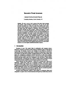
Since id is the neutral element, we have id; ρ = ρ; id = ρ for all ρ ∈ M(A). To use boxes for checking inclusion, we have to retrieve the words represented by a box. A box represents the set of all words that yield the prescribed effect. We assign to ρ ∈ B(A) u u the language L(ρ) of all words u ∈ T + that satisfy q → q 0 for all (q, q 0 , ∗) ∈ ρ and q →f q 0 for all (q, q 0 , 1) ∈ ρ. There is a u-labeled path from q to q 0 iff the box contains a corresponding triple (where the label is not important). Moreover, one of the u-labeled paths can visit a final state iff this is required. n o u u L(ρ) = u ∈ T + for all (q, q 0 , ∗) ∈ ρ : q → q 0 and for all (q, q 0 , 1) ∈ ρ : q →f q 0 To the element id we assign the singleton language L(id) := {ε}. The empty word cannot be lifted to an infinite word through ω-iteration, and therefore has to be handled with care. We use function ρ : T ∗ → M(A) to abstract a word w ∈ T ∗ to the unique box ρw representing it in the sense that w ∈ L(ρw ). Note that ρuv = ρu ; ρv . This means the boxes with a non-empty language can be computed from the boxes of the letters ρa , where ρa contains (q, q 0 , i) iff there is an a-labeled edge from q to q 0 . We have i = 1 iff q or q 0 is final. In particular, the image ρT ∗ is precisely the set of boxes ρ with L(ρ) 6= ∅. Figure 1 illustrates the representation of words of Büchi automaton Aex by boxes. The representation of finite words by boxes can be lifted to infinite words. We recall two results that date back to [28]. The first result states that every infinite word is contained ω in a composition L(τ ).L(ρ) of the languages of only two boxes. The proof uses Ramsey’s theorem in a way similar to Theorem 10, and indeed inspired our result. The second result

6


req ack, s, t

q0

q1

req, s, t


ε id = ρε

ack

ρreq

ρack

ρs = ρt

ρack.req

Figure 1 The automaton Aex and its boxes. The upper dash on each side of a box represents state q0 , the lower dash represents q1 . A dot on the dash marks that a final state has been visited.

states that a language L(τ ).L(ρ) is either contained in Lω(A) or it is disjoint from Lω(A). It follows from the definition of box languages. Together, one can understand the set of ω languages L(τ ).L(ρ) as a finite abstraction of T ω that is precise enough wrt. inclusion in ω L(A). We refer to the languages L(τ ).L(ρ) included in L(A) as the cover of L(A). ω

I Lemma 5. (1) For every w ∈ T ω there are τ, ρ ∈ B(A) with w ∈ L(τ ).L(ρ) . ω ω (2) Let ρ, τ ∈ B(A). We have L(τ ).L(ρ) ⊆ Lω(A) or L(τ ).L(ρ) ⊆ Lω(A) . ω

We compute the set of boxes summarizing the effect of the words derivable from a nonterminal as the least solution to a system of inequalities. The system is interpreted over the complete lattice (P(M(A)), ⊆). For two sets of boxes S, R ⊆ M(A), we define their composition S; R = {τ ; ρ | τ ∈ S, ρ ∈ R} to be the set of all pairwise compositions. There are two types of variables, ΛX and ∆X,Y for all non-terminals X and Y . The solution to a variable ΛX will contain the boxes for the words derivable from X. The task of ∆X,Y is to additionally remember the rightmost non-terminal. This means we compute the boxes of all words w with X ⇒∗ wY . The point is that the lasso-finding test has to match successive non-terminals Y in the right-infinite derivation. The inequalities for the variables ΛX are as follows. For every rule X → α, we require ΛX ≥ Λα . Here, we generalize the notation Λ from non-terminals to sentential forms by setting Λε := {id}, Λa := {ρa }, and Λαβ := Λα ; Λβ . For the second set of variables, there is a base case. For every non-terminal Y , we require ∆Y,Y ≥ {id}. The empty word takes Y to Y and is represented by id. For every pair of non-terminals X, Y and for every edge (X, α, Z) in the ω-graph, we have the inequality ∆X,Y ≥ Λα ; ∆Z,Y . To understand the requirement, assume Z = Y and thus ∆Y,Y ≥ {id}. Then the solution to ∆X,Y indeed contains the boxes of the words w with X ⇒ αY ⇒∗ wY . If Z 6= Y , we compose the solution to Λα with further boxes found on the way from Z to Y . The least solution to the above system of inequalities is computed as the least fixed point of the function on the product domain induced by the right-hand sides. A standard Kleene iteration [9] and more efficient methods like chaotic iteration [26] apply. We use σX and σX,Y to denote the least solution to ΛX and ∆X,Y , respectively. Again, we generalize the notation to sentential forms, σα . I Example 6. In our running example, the system of inequalities (for Gex and Aex ) is ΛX ≥ {ρreq }; ΛY ; {ρack }

ΛY ≥ {ρs }; ΛY ; {ρt }

∆X,X ≥ ΛX ; ∆X,X

∆X,X ≥ {id}

ΛX ≥ ΛX ; ΛX

ΛY ≥ {id}

∆X,Y ≥ ΛX ; ∆X,Y

∆Y,Y ≥ {id}

The least solution is σX = {ρack }, σY = {id, ρs }, σX,X = {id, ρack }, σY,Y = {id}, σX,Y = ∅, and σY,X = ∅. The following lemma states the indicated correspondence between the solution and the words in the language.


7

I Lemma 7. σX = ρL(X) and σX,Y = ρL(P(X,Y )) = {ρw | w ∈ L(p), p ∈ P(X, Y )}. In particular, all occurring boxes have a non-empty equivalence class. With the semantical results at hand, we can develop our lasso-finding algorithm. Lassos, a ω notion proposed in [14], denote elements L(τ ).L(ρ) in the cover of L(A) (see the discussion before Lemma 5). Intuitively, a pair of boxes (τ, ρ) forms a lasso if box ρ, when seen as a graph with the set of states as its vertex set, contains a strongly connected component that is accepting (contains a final state) and that is reachable from the first box. I Definition 8. A pair (τ , ρ) ∈ M(A) × M(A) is a lasso, if either ρ = id holds or there are states q, q 0 ∈ Q, a transition (q0 , q, x) ∈ τ , a path from q to q 0 in ρ, and an accepting path from q 0 to q 0 (a loop) in ρ. The definition is illustrated to the right. With the aforementioned graph-theoretic interpretation of lassos, it can be checked in linear time whether a pair of boxes actually forms a lasso. Lassos characterize the cover in the following sense.

q0

τ

q

ρ∗

q0

ρ∗

I Lemma 9. Let ρ, τ ∈ M(A) with L(τ )L(ρ) 6= ∅. Then L(τ )L(ρ) ⊆ Lω(A) holds if and only if (τ, ρ) is a lasso. ω

ω

Note that if ρ = id then L(τ )L(ρ) = ∅. Hence, we can assume that the first case in the definition of lassos does not apply. It is routine to check the correspondence. Let us consider Aex again and choose τ = ρreq = {(q0 , q1 , 1), (q1 , q1 , 0)} and ρ = ρs = {(q0 , q0 , 1), (q1 , q1 , 0)}. The only transition in τ starting from initial state q0 is (q0 , q1 , 1) and the only accepting loop in ρ is (q0 , q0 , 1). However, there is no path from q1 to q0 in ρ. Thus, ω (τ, ρ) is not a lasso and L(τ )L(ρ) 6⊆ Lω(Aex ). ω

I Theorem 10. The inclusion Lω(G) ⊆ Lω(A) holds if and only if for every non-terminal X ∈ N , for every box τ in σS,X and for every box ρ in σX,X , the pair (τ, ρ) is a lasso. One may check that using the grammar Gex from our running example and the automaton Aex from Figure 1, the condition is fulfilled and inclusion holds, i.e. Lω(Gex ) ⊆ Lω(Aex ).

4

Liveness Synthesis

Two player games with perfect information form the theory behind synthesis problems. In this section, we generalize a recent algorithm for solving context-free games with regular inclusion as the winning condition [16] to ω-context-free games with ω-regular winning conditions. An ω-context-free game is given as a context-free grammar G = (N, T, P, S) where the non-terminals N = N ∪· N are partitioned into the non-terminals owned by player prover and the ones owned by player refuter . The winning condition is defined by a Büchi automaton A. Player will win the game if she enforces the derivation of an infinite word not in the language of A. Player will win the remaining plays. Formally, the game induces a game arena, a directed graph defined as follows. (1) The set of vertices is the set of all sentential forms ϑ = (N ∪· T )∗ . (2) A vertex is owned by the player owning the leftmost non-terminal. Terminal words are owned by refuter. (3) The edges are defined by the left-derivation relation: If α = wXβ with β 6= ε, then α → γ in the game arena if α ⇒ γ by replacing X. If α = wX, i.e. X is the leftmost and only non-terminal, then α → γ if α ⇒ γ by a left-derivation using a rule X → ηY having a rightmost non-terminal. A (maximal) play of the game is a path in the game arena that is either infinite or ends in

8



a deadlock, i.e. in a vertex that has no successor. We think of the moves originating from vertices owned by resp. as chosen by prover resp. refuter. The goal of refuter is to derive an infinite word outside Lω(A), we also say that refuter plays a non-inclusion game. We define the infinite word derived by a play as the limit of the sequence of terminal prefixes. Given a sentential form α = wXβ ∈ ϑ, we define its terminal prefix to be w ∈ T ∗ . An infinite play p = α0 , α1 , . . . of the game induces an infinite sequence of such prefixes w0 = prefix(α0 ), w1 = prefix(α1 ), . . ., where each wj itself is a prefix of wj+1 . Assume the words in the sequence of prefixes grow unboundedly, i.e. for any i ∈ N, there is j such that |wj |> i. The limit of the prefixes of p is the infinite word lim prefix(p) defined by lim prefix(p) i = (wj )i , where wj with |wj | > i is an arbitrary terminal prefix. An infinite play p is winning with respect to the non-inclusion winning condition if (1) the prefixes of the positions in p grow unboundedly, and (2) lim prefix(p) 6∈ Lω(A), and (3) positions of shape wX occur infinitely often in p. Otherwise p is winning with respect to the inclusion winning condition. This is in particular the case if p is finite but maximal. Condition (1) enforces that lim prefix(p) is a well-defined infinite word. Condition (3) guarantees that it stems from a right-infinite derivation process. Our goal is to develop an algorithm that, given a grammar and a Büchi automaton, decides whether refuter can win non-inclusion from the initial position S. Our overall strategy, following [29], is to reduce the problem to a finite parity game. The observation behind our reduction is the following. Each play that wins non-inclusion contains infinitely many positions of shape wX. We can therefore split the play into infinitely many parts of finite length, each starting with a position of shape wX. In a first step, we compute for every X a description of all plays from X to sentential forms of the shape uY . In a second step, we combine the information on the finite parts into a finite parity game. Lifting the characterization of finite plays computed in the first step to the infinite plays under study is non-trivial. Our approach is to determinize the given non-deterministic Büchi automaton into a deterministic parity automaton. A deterministic parity automaton (DPA) is a tuple (Q, T, qinit , →, Ω), where Q is a finite set of states, qinit ∈ Q is the initial state, and → : Q × T → Q is the transition function. Rather than final states, Ω : Q → N assigns a priority i ∈ N to each state. We extend the transition function to words and augment it by w the highest occurring priority: We write q →i q 0 if processing w starting in q leads to state q 0 and the highest priority of q, q 0 , and any intermediary state is i. The language Lω(AP ) consists of all words w ∈ T ω such that the highest priority occurring infinitely often on the states in the run of AP on w is even. Non-deterministic Büchi automata can be converted to deterministic Rabin automata [23], which in turn can be transformed to deterministic parity automata, see e.g. [21]. I Theorem 11 ([23, 21]). For an NBA A with n states, one can construct a DPA AP with at most 2O(n log n) states and maximal priority ≤ 2n + 2 so that Lω(A) = Lω(AP ). From now on, we will work with the computed DPA AP = (Q, T, qinit , →, Ω).

4.1

From Context-Free Games to Formulas

Our goal is to employ the characterization of inclusion games over finite words developed in [16]. Semantically, the characterization is given as a positive Boolean formula over a finite set of atomic propositions. The formula captures the tree of all plays starting in a nonterminal by interpreting refuter positions as disjunctions, prover positions as conjunctions, and terminal words as atomic propositions. Algorithmically, the formulas for all non-terminals are computed as the least solution to a system of equations.


9

In the current setting, (1) we have to track the priorities obtained when processing a terminal word and (2) we are given a deterministic rather than a non-deterministic automaton. To reflect (1), we will consider as atomic propositions pairs (p, i) consisting of a state p ∈ Q and a priority i ∈ Ω(Q). Using (2), we define a system of equations with variables ∆qX for each state q ∈ Q and each non-terminal X ∈ N . Intuitively, in the formula for ∆qX w atomic propositions (p, i) represent terminal words w such that X ⇒∗ w and q →i p. In the following, we define the domain and then set up the system of equations. Let pBF(Q × Ω(Q)) be the set of positive Boolean formulas over atomic propositions consisting of a state and a priority. We will assume that the unsatisfiable formula false is also contained in pBF(Q × Ω(Q)). Conjunction ∧ and disjunction ∨ are defined as usual. To simplify the technical development, we evaluate operations involving false on a syntactical level by using the rules F ∨ false = false ∨ F = F and F ∧ false = false ∧ F = false. Assume F represents the plays from state q and non-terminal X, and for each state q 0 the formula Gq0 represents the plays from q 0 and Y . To obtain the formula representing the plays from q and the sentential form XY , we can combine F and the family (Gq0 )q0 ∈Q : A play from XY to a terminal word can be decomposed into a play from XY to wY , and a play from wY to wv. The first part has the same structure as a play from X to w, and the second part is essentially a play from Y to v with w prepended. We think of each atomic w proposition (p, i) in F as describing the behavior of a word w, i.e. q →i p. We obtain the formula imitating this behavior for XY by replacing each atomic proposition (p, i) in F by the formula Gp that describes the effect of Y from p on. To reflect that the highest priority seen while processing wv is the maximum of the priorities seen while processing w and v, we will have to modify the priorities occurring in Gp . We formalize the above discussion in the definitions of the composition operator ; on formulas and the operator : that composes one formula with a family of formulas. Here and in the rest of the paper, we assume that F, F 0 , G, G0 ∈ pBF(Q × Ω(Q)) are formulas, and (Gq )q∈Q and (Hq )q∈Q are families of formulas. Furthermore, (p, i), (p0 , i0 ) ∈ Q × Ω(Q) are atomic propositions and ∗ ∈ {∧, ∨}: (F ∗ F 0 ) : (Gq )q∈Q = F : (Gq )q∈Q ∗ F 0 : (Gq )q∈Q (p, i); (G ∗ G ) = (p, i); G ∗ (p, i); G 0

0

(p, i) : (Gq )q∈Q = (p, i); Gp (p, i); (p0 , i0 ) = (p0 , max{i, i0 }) .

Also here, we handle false on a syntactic level by defining F ; false = false; G = false and false : (Gq )q∈Q = false. The case (F ∗ F 0 ); (p, i) does not occur. We will also need to represent the terminal symbols and ε. Given a state q and a ∈ T , qa a is the formula formed by the atomic proposition (p, i), where q →i p and i = max{Ω(q), Ω(p)}. To handle ε, we define qε to be (q, 0). One might expect the second component to be Ω(q), but setting it to 0 makes the case εω (which is not an infinite word) simpler. To guarantee that a system of equations interpreted over pBF(Q × Ω(Q)) has a unique least solution, we need a partial order on the domain. It has to have a least element and the operations have to be monotonic. Since we deal with Boolean formulas, implication ⇒ is the obvious choice for the order. Unfortunately, it is not antisymmetric, which we will tackle in a moment. The least element is false. Monotonicity is the following lemma. I Lemma 12. The compositions ; and : are monotonic: If F ⇒ F 0 , G ⇒ G0 , and for each q ∈ Q, Gq ⇒ G0q , then F ; G ⇒ F 0 ; G0 and F : (Gq )q∈Q ⇒ F 0 : (G0q )q∈Q . For the solution to be computable, we have to operate on a finite domain. Since we deal with formulas ordered by implication, we can factor them by logical equivalence. This yields a finite domain and takes care of the missing antisymmetry. The order and all operations will be

10



adapted to the domain pBF(QAP × P )/⇔ by applying them to arbitrary representatives. This makes ⇒ a partial order on the equivalence classes, and all other operations are well-defined since they were monotonic with respect to implication. We are now ready to define the system of equations induced by G and AP . To simplify · the notation, we will define ∆qa = qa for a ∈ T ∪{ε}. We extend this to sentential forms by using composition: ∆qαβ = ∆qα : (∆pβ )p∈Q . The following lemma states that this is well-defined and not dependent on the splitting of αβ. I Lemma 13. The composition of families is associative in the following sense: F : (Gq )q∈Q : (Hp )p∈Q = F : Gq : (Hp )p∈Q . q∈Q

For each non-terminal X ∈ and each state q ∈ Q, we have one defining equation (V ∆qη , X ∈ N , ∆qX = WX→η X→η ∆qη , X ∈ N . The resulting system of equations is solved by a standard fixed-point iteration, starting with the equivalence class of false for each component. We define σqX to be the value of ∆qX in the least solution, and we extend this to sentential forms as above: σqa = qa for · a ∈ T ∪{ε}, σqαβ = σqα : (σpβ )p∈Q . To show that the formula σqα indeed describes the behavior of all finite plays from α, we construct strategies that are guided by the formula. Strategies. We fix for each equivalence class of formulas σqα a representative in conjunctive normal form (CNF). (We prove that the development is independent from the choice of the representative.) The conjunctions correspond to the choices of prover during the play. The choices of refuter correspond to selecting one atomic proposition per clause. We formalize the selection process using the notion of choice functions. A choice function on a formula F is a function c : F → Q × Ω(Q) selecting an atomic proposition from each clause, c(K) ∈ K for all K ∈ F . We show that there is a strategy for refuter to derive at least one terminal word having one of the chosen effects on the automaton. In particular, the strategy will only generate finite plays. I Proposition 14. (1) Let K be a clause of σqα . There is a strategy sK for prover such that all maximal plays starting in α that conform to sK are either infinite or end in a terminal w word w such that q →i q 0 and (q 0 , i) ∈ K. (2) Let c be a choice function on σqα . There is a strategy sc for refuter such that all maximal plays starting in α that conform to sc end in a w terminal word w with q →i q 0 and (q, i) ∈ c(σqα ). The proof of Part (2) is a deterministic version of the analogue result in [16]. Since we do not have to guarantee termination of the play, Part (1) it is simpler. Towards Infinite Games. The solution of the system of equations characterizes for each non-terminal X the terminal words w that can be derived from X. For the infinite game, we have to characterize the sentential forms wY that can be derived from X. Since there may be several different non-terminals Y such that a sentential form wY is reachable from X, we store the target non-terminal in the atomic propositions. For F ∈ pBF(Q × Ω(Q)) and a non-terminal Y , we define F.Y to be the formula in pBF(Q × Ω(Q) × N ) that is obtained by adding Y as a third component in every atomic proposition. With ∗ ∈ {∨, ∧}, we set (F ∗ F 0 ).Y = F.Y ∗ F 0 .Y ,

(q, i).Y = (q, i, Y ) .

R. Meyer, S. Muskalla, and E. Neumann For each non-terminal X, we collect all rules X → ηY with a non-terminal Y as their rightmost symbol. We represent the behavior of η by the previously computed formulas σqη and attach Y as described above. The resulting formulas are combined using disjunction or conjunction, depending on the owner of X. Given a non-terminal X and a state q ∈ Q, we define the extended solution for qX to be e σqX

=

(V W

X→ηY

σqη .Y,

X ∈ N ,

X→ηY

σqη .Y,

X ∈ N ,

If no rule of the shape X → ηY exists, the formula is false. The latter is to model that prover wins in this case, independently of who owns X. e . There is a strategy seK for prover such I Proposition 15. (1) Let K be a clause of σqX that all maximal plays starting in X that conform to seK are either infinite without visiting a w sentential form of shape wY , or they visit a sentential form of shape wY such that q →i q 0 e and (q 0 , i, Y ) ∈ K. (2) Let c be a choice function on σqX . There is a strategy sec for refuter such that all maximal plays starting in X that conform to sec visit a sentential form of shape w e wY such that q →i q 0 and (q, i, Y ) ∈ c(σqX ).

4.2

From Formulas to a Parity Game

It remains to combine the formulas for finite plays to obtain a characterization of the infinite plays. We model the infinite plays as an infinite sequence of alternations: First, prover chooses a clause from the formula for X, which fixes her strategy for the following finite part. Second, refuter chooses an atomic proposition from the selected clause, which fixes the derived sentential form wY . Instead of storing the (unboundedly growing) prefixes w explicitly, we only store the target non-terminal, the state transition of AP while processing w, and the highest priority occurring during the transition. Modeling the game like this leads to a parity game on a finite graph. A parity game P = (V = V ∪· V , E, Ω) is a directed graph with an ownership partitioning of the vertices and a function Ω : V → N that assigns to each vertex a priority. We will assume that the parity game is deadlock-free. A maximal play is an infinite path in the graph. It is won by player if the highest priority occurring infinitely often on the vertices in the play is even; won by player otherwise. I Theorem 16 (Positional Determinacy of Parity Games, [30]). Given a parity game P, there is a decomposition of the vertices V = W ∪· W and there are positional strategies s : V → V , s : V → V such that s is winning from all positions in W and s is winning from all positions in W . I Definition 17. The parity game PG,AP induced by the context-free grammar G and the DPA AP is (V = V ∪· V , E, Ω). The vertices V = {qX | q ∈ Q, X ∈ N } represent the formulas. They are owned by prover because prover is allowed to pick a clause. The vertices of refuter V = V clause ∪· V helper are of two types. Since refuter should select an atomic proposition, e she owns the vertices V clause = qXK q ∈ Q, X ∈ N, K ∈ σqX representing the clauses. helper e The helper vertices V = (qXK, i, pY ) q ∈ Q, X ∈ N, K ∈ σqX , (p, i, Y ) ∈ K will be used to keep track of the priority that is seen while processing the terminal prefix w that is created by going from X to wY . The edges connect non-terminals to clauses, and clauses to the next formula via the helper vertices:

11

12

Liveness Verification and Synthesis: E=


e (qX, qXK) q ∈ Q, X ∈ N, K ∈ σqX

e (qXK, (qXK, i, pY )), ((qXK, i, pY ), pY ) q ∈ Q, X ∈ N, K ∈ σqX , (p, i, Y ) ∈ K e ∪· (qXK, qXK) q ∈ Q, X ∈ N, K ∈ σqX ,K = ∅ . The last part takes care of the empty clause which occurs iff the formula is equivalent to false. The priority function is zero but on the helper vertices, where it returns the priority given by the selected atomic proposition: Ω(qX) = Ω(qXK) = 0, Ω((qXK, i, pY )) = i. ∪·

We are now able to state the correspondence between the ω-context-free game of interest and the constructed parity game. I Theorem 18 (Determinacy of ω-Context-Free Games). Prover resp. refuter has a winning strategy for the ω-regular inclusion game from S iff she wins the parity game from q0 S. Proof Sketch. Using Theorem 16 on the positional determinacy of parity games, exactly one of the players wins the parity game from q0 S, and she has a positional winning strategy. We use this positional winning strategy to construct a winning strategy for the ω-context-free game. To this end, we establish a correspondence between the play of the parity game and the run of AP on an infinite word derived in the ω-context-free grammar by following the play. The key idea is that a winning strategy for the parity game for prover resp. refuter fixes clauses resp. choice functions. Using these clauses resp. choice functions, we can apply Proposition 15 to obtain a strategy for the finite part of the ω-context-free game that is played until the next sentential form represented in the parity game (by a vertex) is found. We make this precise in Section C.2. J

4.3

Complexity

We show that deciding whether refuter has a winning strategy for ω-regular non-inclusion from position S is a 2EXPTIME-complete problem. Moreover, the algorithm presented in this section achieves this optimal time complexity. Our proof of the lower bound works by showing that the case of finite inclusion games can be seen a special case of the problem under consideration here. Solving finite context-free games has been shown to be a 2EXPTIME-complete problem in [20]. I Theorem 19. Solving ω-context-free games is 2EXPTIME-hard. We summarize the algorithm outlined in this section: (1) Construct the deterministic parity automaton AP . (2) Construct and solve the system of equations. (3) Extend the solution σ to obtain σ e . (4) Construct the finite parity game PG . (5) Check which player wins PG from q0 S. I Theorem 20. Given an ω-context-free game and an initial |Q| position, the algorithm outlined c1 2 |G|c2 above decides which player wins in time O 2 ·2 for some constants c1 , c2 ∈ N.


References 1

2

3 4

5 6 7 8 9 10 11 12 13 14 15 16 17 18 19 20 21 22 23 24

P. A. Abdulla, Y.-F. Chen, L. Clemente, L. Holík, C.-D. Hong, R. Mayr, and T. Vojnar. Simulation subsumption in Ramsey-based Büchi automata universality and inclusion testing. In CAV, volume 6471 of LNCS, pages 132–147. Springer, 2010. P. A. Abdulla, Y.-F. Chen, L. Clemente, L. Holík, C.-D. Hong, R. Mayr, and T. Vojnar. Advanced Ramsey-based Büchi automata inclusion testing. In CONCUR, volume 6901 of LNCS, pages 187–202. Springer, 2011. H. Björklund, M. Schuster, T. Schwentick, and J. Kulbatzki. On optimum left-to-right strategies for active context-free games. In ICDT, pages 105–116. ACM, 2013. A. Bouajjani, J. Esparza, and O. Maler. Reachability analysis of pushdown automata: Application to model-checking. In CONCUR, volume 1243 of LNCS, pages 135–150. Springer, 1997. C. Broadbent, A. Carayol, M. Hague, and Olivier O. Serre. C-SHORe: A collapsible approach to higher-order verification. ACM SIGPLAN Notices, 48(9):13–24, 2013. J. R. Büchi. On a Decision Method in Restricted Second Order Arithmetic, pages 425–435. Springer, 1990. T. Cachat. Symbolic strategy synthesis for games on pushdown graphs. In ICALP, volume 2380 of LNCS, pages 704–715. Springer, 2002. R. S. Cohen and A. Y. Gold. Theory of ω-languages (i and ii). JCSS, 15(2):169–184, 185–208, 1977. B. A. Davey and H. A. Priestley. Introduction to Lattices and Order. CUP, 1990. A. Farzan, Z. Kincaid, and A. Podelski. Proof spaces for unbounded parallelism. In POPL, pages 407–420. ACM, 2015. A. Farzan, Z. Kincaid, and A. Podelski. Proving liveness of parameterized programs. In LICS. IEEE, 2016. Azadeh Farzan, Zachary Kincaid, and Andreas Podelski. Proofs that count. In POPL, pages 151–164. ACM, 2014. O. Finkel. Topological properties of omega context-free languages. Theor. Comp. Sci., 262(1):669–697, 2001. S. Fogarty and M. Y. Vardi. Efficient Büchi universality checking. In TACAS, volume 6015 of LNCS, pages 205–220. Springer, 2010. M. Heizmann, J. Hoenicke, and A. Podelski. Nested interpolants. In POPL, pages 471–482. ACM, 2010. L. Holík, R. Meyer, and S. Muskalla. Summaries for context-free games. In FSTTCS, LIPIcs. Dagstuhl, 2016. To appear, https://arxiv.org/abs/1603.07256. Lukás Holík and Roland Meyer. Antichains for the verification of recursive programs. In NETYS, volume 9466 of LNCS, pages 322–336. Springer, 2015. M. Linna. On ω-sets associated with context-free languages. Inf. Cont., 31(3):272–293, 1976. Z. Long, G. Calin, R. Majumdar, and R. Meyer. Language-theoretic abstraction refinement. In FASE, volume 7212 of LNCS, pages 362–376. Springer, 2012. A. Muscholl, T. Schwentick, and L. Segoufin. Active context-free games. Theory of Computing Systems, 39(1):237–276, 2005. N. Piterman. From nondeterministic B˘"chi and Streett automata to deterministic parity automata. Log. Meth. Comput. Sci., 3(3), 2007. T. Reps, S. Horwitz, and M. Sagiv. Precise interprocedural dataflow analysis via graph reachability. In POPL, pages 49–61. ACM, 1995. S. Safra. On the complexity of ω-automata. In FOCS, SFCS, pages 319–327. IEEE, 1988. Jacques Sakarovitch. Elements of Automata Theory. Cambridge University Press, 2009.

13

14


25 26 27 28

29 30


M. Schuster and T. Schwentick. Games for active XML revisited. In ICDT, volume 31 of LIPIcs, pages 60–75. Dagstuhl, 2015. H. Seidl, R. Wilhelm, and S. Hack. Compiler Design - Analysis and Transformation. Springer, 2012. M. Sharir and A. Pnueli. Two approaches to interprocedural data flow analysis. Technical Report 2, New York University, 1978. A. P. Sistla, M. Y. Vardi, and P. Wolper. The complementation problem for B˘"chi automata with applications to temporal logic. In ICALP, volume 194 of LNCS, pages 217–237. Springer, 1985. I. Walukiewicz. Pushdown processes: Games and model-checking. Information and Computation, 164(2):234 – 263, 2001. W. Zielonka. Infinite games on finitely coloured graphs with applications to automata on infinite trees. Theor. Comp. Sci., 200(1-2):135–183, 1998.


A

15

Details on Section 2

One direction of the proof of Proposition 2 is immediate. We prove it in the form of the following proposition. I Proposition 21. Let L ⊆ T ω be a ω-context-free language. Then there is a CFG G such that L = Lω(G). Proof. We may assume [ L= Vi Uiω i=1,...,n

and there are CFGs GVi = (NVi , T, PVi , SVi ),

GUi = (NUi , T, PUi , SUi ),

with Vi = L(GVi ) and Ui = L(GUi ) for all i such that all sets of non-terminals are pairwise disjoint. We construct a new grammar G = (N, Σ, P, S) with N = {S} ∪· S S {Ri | i = 1, ..., m} ∪· · i=1,...,n NUi ∪· · i=1,...,n NVi and P = {S → SVi Ri | i = 1, ..., m} ∪· S S {Ri → SUi Ri | i = 1, ..., m} ∪· · i=1,...,n PUi ∪· · i=1,...,n PVi . L = Lω(G) is easy to see. J Intermediary Infiniteness. A grammar is supposed to generate the infinite computations of a recursive program, and a rule X → aY Z should be understood as procedure X executing action a, calling procedure Y , and after Y has returned continuing with procedure Z. Our restriction to the right-infinite derivations allows procedure Z to run forever, but for Y we only consider finite executions. The reader may argue that we should also consider the infinite executions of Y . Interestingly, our restriction to the right-infinite derivations increases the expressiveness of the language class compared to a definition that closes the ω-language under intermediary infiniteness. The alternative definition yields a subclass of the ω-context-free languages as one can always add shortened rules to a given grammar that reflect intermediary infiniteness. In the example, one would just have to add the rule X → aY to also reflect the fact that the program may do its infinite computation without returning from procedure Y . To see that the inclusion is strict, consider the language L = (ani bni )ω with ni ∈ N for all i. The language containing L would also contain aω 6∈ L. Proof of Lemma 4. For non-terminals A, B ∈ N and a set M ⊆ N of non-terminals, we M define P(A, B) to be the set of all finite paths from A to B in the ω-graph such that all occurring intermediary vertices are in M . We show that the corresponding language [ M L P(A, B) = L(p) P ∈P(A,B)M

is context-free by induction on the size of M . This proves that

S

p∈P(X,Y )

L(p) is context-free

since P(X, Y ) = P(X, Y ) . ∅ Case M = ∅: All paths in P(A, B) have length at most one. If A = B, the corresponding language contains and all elements of the context-free languages L(α) for all self-loops (A, α, A). If A 6= B, the corresponding language contains all elements of the context-free languages L(α) for all edges (A, α, B). Since there are only finitely many of those edges, and context-free languages are closed under finite unions, the language corresponding to ∅ P(A, B) is context-free. N

16



Case M = 6 ∅: Let us first consider the special case of cycles (i.e. A = B) and A ∈ M . Any cycle in which A occurs as intermediary vertex can be decomposed into several cycles, such that A does not occur as intermediary vertex in any of those. We can use this to obtain the representation ∗ ∗ M M \{A} L P(A, A) = ∪c∈P(A,A)M \{A} L(c) = L P(A, A) which is context-free by induction and since context-free languages are closed under Kleeneiteration. In the general case, any path p from A to B has either no repeating intermediary vertex, i.e. it is simple, or there is an intermediary vertex C occurring several times. In the latter case, it can be decomposed, p = pAC cC pCB where pAC is a path from A to C, pC a cycle in C, and a pCB a path from C to B. We can assume that C does not occur as intermediary vertex in pAC and pCB , and as before, we can decompose cC = c1 c2 . . . ck into finitely many cycles such that C does not occur in any of them as intermediary vertex. Altogether, we retrieve the representation ! ! ∗ [ [ M0 M0 M0 L(p) ∪ L P(A, C) L P(C, C) L P(C, B) p∈P(A,B)M p simple

C∈N

where M 0 = M \ {C}. The first part is context-free since there are only finitely many simple paths. The second part is a finite union of concatenations of context-free languages (by induction and closure under Kleene-iteration). Altogether, this shows that L P(A, B)

M

B

is context-free.

J

Details on Section 3

Proof of Lemma 7. For the proof of σX = ρL(X) , we refer to the proof of Lemma 3 in [17]. It remains to prove σX,Y = ρL(P(X,Y )) = {ρw | w ∈ L(p), p ∈ P(X, Y )}. Assume there is a word in w ∈ L(p), p ∈ P(X, Y ). Let p = α0 . . . αk be a decomposition of the path into its edges. By plugging in the inequalities into each other along the path, one can see that σX,Y ≥ σα0 ; ...; σαk ; {id} = σα0 ; ...; σαk . We can write w = w0 ...wm such that for each i, wi ∈ L(αi ). By the first part of the Lemma, we have σαi = {ρw | w ∈ L(αi )} for each i, in particular ρwi in σαi . By the definition of the composition of sets of boxes and the above inequality, we then also have ρw ∈ σX,Y . Assume there is a box ρ in σX,Y . We prove using induction that all boxes in σX,Y j have corresponding words in L(P(X, Y )), where σ j is the intermediary solution after the j th -step of Kleene iteration. Since σX,Y = σX,Y j0 for some j0 , this proves the claim. If the ρ entered the solution in the first iteration we have ρ = id and we are done. If it entered the solution in step j > 0, then there is some edge (X, α, Z) in the ω-graph such that ρ ∈ σα ; σZ,Y j−1 , where σ j−1 is the solution after the (j − 1)th iteration. There are boxes τ1 ∈ σα , τ2 ∈ σZ,Y j−1 such that ρ = τ1 ; τ2 . By the first part of the theorem, there is a word w1 such that w1 ∈ L(α) with ρw1 = τ1 . By induction, there is a word w2 such that w2 ∈ L(P(Z, Y )) with ρw2 = τ2 . Then w = w1 w2 is a word in L(P(X, Y )) with ρw = ρw1 ; ρw2 = τ1 ; τ2 = ρ. J


17

Proof of Lemma 9. Note that if ρ = id, then τ ρω = ∅. Assume (τ, ρ) is a lasso, then there is an edge (q0 , q, x) ∈ τ , a path p from q to some q 0 in ρ and a loop c from q 0 to q 0 in ρ such that at least one edge on the loop is labeled by one. Let k be the length of p and let m be the length of c. ω Assume w ∈ L(τ )L(ρ) , then there is a decomposition w = w(0) w(1) . . . with τ = ρw(0) and ρ = ρw(1) = ρw(i) for all i > 0. Then the following sequence can be refined to a run by inserting intermediary states: w(0)

w(1) ...w(1+k)

w(1+k+1) ...w(1+k+c)

w(1+k+c+1) ...w(1+k+2·c)

q0 → q −−−−−−−−→ q 0 −−−−−−−−−−−−−→ q 0 −−−−−−−−−−−−−−−→ . . . Since at least one edge occurring in the loop is labeled by 1, one can refine the sequence to an accepting run that visits infinitely many final states. This shows w ∈ Lω (A). ω Let us now assume w ∈ L(τ )L(ρ) , w ∈ Lω (A), i.e. there is an accepting run of w on A. (0) (1) Let w = w w ... with τ = ρw(0) and ρ = ρw(1) = ρw(i) for all i > 0. We fix an arbitrary accepting run of A on w. Let q (i) be the state of A in this run after processing w(i) for each i. We define q = q (0) and q 0 to be the first state which occurs infinitely often in the sequence of the q (i) . Let p be the path from q (0) to q 0 in ρ. There has to be an occurrence of q 0 , say q (j) , such that there is a final state between the first occurrence of q 0 and q (j) . This proves that ρ contains a loop c from and to q 0 in which at least one edge is labeled by 1. The membership of the words in the languages of the boxes guarantees the existence of p and c. The transition (q0 , q (0) , ∗) ∈ τ , the path p and the loop c prove that (τ, ρ) is a lasso. J Proof of Theorem 10. For the implication from right to left, we show that whenever the inclusion fails, there is a non-terminal X, a box τ ∈ σS,X , and a box ρ ∈ σX,X such that (τ, ρ) is no lasso. Consider the word w ∈ Lω(G) \ Lω(A). By definition of Lω(G), there is a decomposition w = w(0) w(1) w(2) ... and an infinite sequence of rules S → α0 X1 , X1 → α1 X2 , . . . so that w(j) ∈ L(αj ) for all j. Let X be a non-terminal which occurs infinitely often in the sequence of the Xi . Such an X exists as there are only finitely many non-terminals. We create a new decomposition w = v (0) v (1) v (2) ... such that in the sequence of rules above, v (0) takes us from S to X for the first time, and each v (j) for j > 0 takes us from X to X. To this decomposition, we apply Ramsey’s theorem which states the following. Every (undirected) infinite complete graph that has a finite edge coloring contains an infinite complete monochromatic subgraph. For the application, define the labeled complete graph to have vertex set N and coloring (for all edges {i, j} with i < j): c({i, j}) = ρvi ; ρvi+1 ; ...; ρvj−1 Ramsey’s theorem yields an infinite complete subgraph such that all edges have the same color. Let S = {s0 , s1 , ...} be the vertex set of this subgraph, with s0 < s1 < . . . This vertex set yields a new decomposition of the word: w = u(0) u(1) u(2) ...

18



with u(0) = v (0) v (1) ...v (s0 −1)

and

u(i) = v (si ) v (si +1) ...v (si+1 −1)

for all i > 0 .

Word u(0) takes us from S to X and all other u(i) take us from X to X. We define τ = ρu(0) and ρ = ρu(1) . Note that since all edges have the same color, we have ρ = ρu(i) for all i > 0. By construction, τ ∈ σS,X and ρ ∈ σX,X . Since w 6∈ Lω(A), we know that (τ, ρ) is no lasso by Lemma 9. For the implication from left to right, assume the inclusion holds, but there are τ ∈ σS,X and ρ ∈ σX,X that do not form a lasso. By Lemma 7, all boxes in σX,Y have non-empty equivalence classes. We also know that ρ = 6 id, since otherwise we would have considered the ω pair a lasso by definition. Hence, there is an infinite word w ∈ L(τ )L(ρ) . By Lemma 7 and 3, this word is also in Lω(G). But by Lemma 9 and Lemma 5, w 6∈ Lω(A), which contradicts the assumption that the inclusion holds. J

C C.1

Details on Section 4 Details on Subsection 4.1

Proof of Lemma 12. We prove the part about : . The proof for the monotonicity of ; is analogous. The proof proceeds in phases (1) to (3) so that the claim in each phase is proven under the assumption of the claim proven in the previous phase. Let {∗, ¯∗} = {∧, ∨}. In the following, we will use ∗ and ¯ ∗ as syntactic parts of formulas as well as to connect statements in the proof. (1) First, we prove the lemma for the case when F, F 0 ∈ Q × P . In this case, F = F 0 = (p, i) and thus F : (Gq )q∈Q = (p, i); Gp = F 0 : (G0q )q∈Q . (2) Next, we assume that F 0 ∈ Q × Ω(Q) and F is an arbitrary formula. We prove the statement by induction on F . Base case: F ∈ Q × Ω(Q), hence (1) proves the statement. Induction step: Let F = F1 ∗ F2 . Note that the Boolean formulas (a ∗ b) ⇒ c and (a ⇒ c) ¯ ∗ (b ⇒ c) are equivalent, called Equivalence (i) in the following. By the Equivalence (i), we get (F1 ⇒ F 0 ) ¯∗ (F2 ⇒ F 0 ). Therefore, by the induction hypothesis, (F1 : (Gq )q∈Q ⇒ F 0 : (G0q )q∈Q ) ¯∗ (F2 : (Gq )q∈Q ⇒ F 0 : (G0q )q∈Q ). This is by (i) equivalent to (F1 : (Gq )q∈Q ∗ F2 : (Gq )q∈Q ) ⇒ F 0 : (G0q )q∈Q . By the definition of :, this shows F : (Gq )q∈Q ⇒ F 0 : (G0q )q∈Q . (3) We assume that both F, F 0 are arbitrary formulas. We prove the statement using induction on the structure of F 0 . Base case: F 0 ∈ Q × Ω(Q), hence the statement is proven by (2). Induction step: Let F 0 = F10 ∗ F20 . By the general equivalence of the Boolean formulas a ⇒ (b ∗ c) and (a ⇒ b) ∗ (a ⇒ c), called Equivalence (ii) in the following, we get (F ⇒ F10 ) ∗ (F ⇒ F20 ). Therefore, by the induction hypothesis, (F : (Gq )q∈Q ⇒ F10 : (G0q )q∈Q ) ∗ (F : (Gq )q∈Q ⇒ F20 : (G0q )q∈Q ) holds. Again by (ii), we get F : (Gq )q∈Q ⇒ (F10 : (G0q )q∈Q ∗ F20 : (G0q )q∈Q ). This is F : (Gq )q∈Q ⇒ F 0 : (G0q )q∈Q by definition. J Proof of Lemma 13. The proof proceeds in phases (1) to (3) so that the claim in each phase is proven under the assumption of the claim proven in the previous phase.

R. Meyer, S. Muskalla, and E. Neumann (1) We first show that ((q 0 , i); (q, j)) : (Hp )p∈Q = (q 0 , i); ((q, j) : (Hp )p∈Q ). To this end, note that: ((q 0 , i); (q, j)) : (Hp )p∈Q = (q, max(i, j)); Hq , (q 0 , i); ((q, j) : (Hp )p∈Q ) = (q 0 , i); ((q, j); Hq ) . We use structural induction on Hq to prove this equality. Base case: Let Hq = (p, k). Then we have (q, max(i, j)); Hq = (q, max(i, j)); (p, k) = (p, max(i, j, k)) = (q 0 , i); (p, max(j, k)) = (q 0 , i); ((q, j); (p, k)) = (q 0 , i); ((q, j); Hq ) . Induction step: Let Hq = H1 ∗ H2 , with ∗ ∈ {∨, ∧}. Thus, (q, max(i, j)); (H1 ∗ H2 ) = (q, max(i, j)); H1 ∗ (q, max(i, j)); H2 = (q 0 , i); ((q, j); H1 ) ∗ (q 0 , i); ((q, j); H2 )

IH

= (q 0 , i); ((q, j); H1 ∗ (q, j); H2 ) = (q 0 , i); (q, j)(H1 ∗ H2 ) . (2) We show that ((q 0 , i) : (Gq )q∈Q ) : (Hp )p∈Q = (q 0 , i) : (Gq : (Hp )p∈Q )q∈Q . Note that ((q 0 , i) : (Gq )q∈Q ) : (Hp )p∈Q = ((q 0 , i); Gq0 ) : (Hp )p∈Q , (q 0 , i) : ((Gq )q∈Q : (Hp )p∈Q ) = (q 0 , i); (Gq0 : (Hp )p∈Q ) . We proceed by structural induction on Gq0 . Base case: Gq0 = (q, j) holds and thus (1) proves the claim. Induction step: Assume Gq = G1 ∗ G2 for ∗ ∈ {∨, ∧}. Then we can derive that ((q 0 , i); (G1 ∗ G2 )) : (Hp )p∈Q = ((q 0 , i); G1 ∗ (q 0 , i); G2 )) : (Hp )p∈Q = ((q 0 , i); G1 ) : (Hp )p∈Q ∗ ((q 0 , i); G2 )) : (Hp )p∈Q = (q 0 , i); (G1 : (Hp )p∈Q ) ∗ (q 0 , i); (G2 : (Hp )p∈Q )

IH

= (q 0 , i); (G1 : (Hp )p∈Q ∗ G2 : (Hp )p∈Q ) = (q 0 , i); ((G1 ∗ G2 ) : (Hp )p∈Q ) . (3) Let now (Gq )q∈Q and (Hq )q∈Q be arbitrary families. We prove the statement by induction on the structure of F . Base case: F = (q 0 , i) ∈ Q × Ω(Q) and (2) proves the statement.

19

20



Induction step: Assume F = F1 ∗ F2 for ∗ ∈ {∨, ∧}. Then, we have (F : (Gq )q∈Q ) : (Hp )p∈Q = ((F1 ∗ F2 ) : (Gq )q∈Q ) : (Hp )p∈Q = (F1 : (Gq )q∈Q ∗ F2 : (Gq )q∈Q ) : (Hp )p∈Q = (F1 : (Gq )q∈Q ) : (Hp )p∈Q ∗ (F2 : (Gq )q∈Q ) : (Hp )p∈Q = F1 : ((Gq )q∈Q : (Hp )p∈Q ) ∗ F2 : ((Gq )q∈Q : (Hp )p∈Q )

IH

= (F1 ∗ F2 ) : ((Gq )q∈Q : (Hp )p∈Q ) = F : ((Gq )q∈Q : (Hp )p∈Q ), which proves the claim.

J

Conjunctive Normal Form. A formula in CNF is a conjunction of clauses, each clause being a disjunction of atomic propositions. We use set notation and write clauses as sets of atomic propositions and formulas as sets of clauses. Identify true = {} and false = {{}}. Since our formulas are negation-free, implication has a simple characterization. I Lemma 22. F ⇒ G if and only if there is j : G → F so that j(H) ⊆ H for all H ∈ G. Proof. The implication from right to left is immediate. Assume F ⇒ G but there is no map j as required. Then there is some clause H ∈ G so that for every clause C ∈ F we find a variable xC ∈ C with xC ∈ / H. Consider the assignment ν(xC ) = true for all xC and ν(y) = false for the remaining variables. Then ν(F ) = true. At the same time, ν(G) = false as ν(H) = false. This contradicts the assumption F ⇒ G, which means ν(F ) = true implies ν(G) = true for every assignment ν. J Disjunctions and compositions can be transformed to CNF by applying distributivity. I Lemma 23. (1) F ∨ G ⇔ {K ∪ H | K ∈ F, H ∈ G}, (3) F : (Gq )q∈Q ⇔

[

[

K∈F z:K→∪q∈Q Gq (q,i)7→H∈Gq

(2) F ∧ G ⇔ F ∪ G , [

(p, j); z((p, j))

(p,j)∈K

Proof. (1) is immediate, (2) follows from applying distributivity. We show (3) by structural induction on F . Base case: Let F = (q, i). Then (q, i) : (Gq )q∈Q = (q, i); Gq = {(q, i); K|K ∈ Gq } [ = {(q, i); z(q, i)} . z:{(q,i)}→Gq (q,i)7→H∈Gq


21

Induction step: We need to distinguish two cases. First assume F = F1 ∧ F2 . Then we have (F1 ∧ F2 ) : (Gq )q∈Q = (F1 : (Gq )q∈Q ) ∧ (F2 : (Gq )q∈Q )   [  [  [ (∗) (p, j); z1 ((p, j)) =   K1 ∈F1 z1 :K1 →∪q∈Q Gq (q,i)7→H∈Gq

∪

[

(p,j)∈K1

 

[

K2 ∈F2 z2 :K2 →∪q∈Q Gq (q,i)7→H∈Gq

(p, j); z2 ((p, j))

[

(p,j)∈K2



 

.



In step (∗), we used the induction hypothesis and part (2) of the Lemma. We define a function ( z1 (q, i), if K ∈ F1 z : K → ∪q∈Q Gq , (q, i) 7→ z2 (q, i), else. Using this definition, we can rewrite the last line of the equation to    [  [ [ (p, j); z((p, j)) ,   K∈F1 ∪F2 z:K→∪q∈Q Gq (q,i)7→H∈Gq

(p,j)∈K

which proves the claim. Assume now F = F1 ∨ F2 . Then, (F1 ∨ F2 ) : (Gq )q∈Q = (F1 : (Gq )q∈Q ) ∨ (F2 : (Gq )q∈Q ) (∗)

= {K ∪ K 0 |K ∈ S1 , K 0 ∈ S2 }, with   [ [ [ S1 =  K1 ∈F1 z1 :K1 →∪q∈Q Gq (q,i)7→H∈Gq

S2 =

[

[

K2 ∈F2 z2 :K2 →∪q∈Q Gq (q,i)7→H∈Gq

(p, j); z1 ((p, j))

(p,j)∈K1

 

[

  

(p, j); z2 ((p, j))

(p,j)∈K2



 

.



Therefore,

=

{K ∪ K 0 |K ∈ S1 , K 0 ∈ S2 } [ [ [

[

K1 ∈F1 K2 ∈F2 z1 :K1 →∪q∈Q Gq z2 :K2 →∪q∈Q Gq (q,i)7→H∈Gq (q,i)7→H∈Gq

 

[

(p,j)∈K1



(p, j); z1 ((p, j))

  

∪

 

[



(p,j)∈K2

(p, j); z2 ((p, j))

  

22



Using z as defined above, we can rewrite this as     [ [ [ (p, j); z((p, j)) ,   K1 ∪K2 z:K1 ∪K2 →∪q∈Q Gq K1 ∈F1 ,K2 ∈F2 (q,i)7→H∈Gq

(p,j)∈K1 ∪K2

which proves the claim.

J

Towards a proof of the first part of Proposition 14, we prove the following Lemma. I Lemma 24. Let K be a clause of σqα for α = wXβ. (1) If X ∈ N , there is X → η and a clause K 0 of σqwηβ such that K 0 ⊆ K. (2) If X ∈ N , for all X → η there is a clause K 0 of σqwηβ such that K 0 ⊆ K. Proof. Let q →i p, i.e. p is the unique state in which AP is after processing w from q. Let F = σqwXβ . We assume that X → η1 , . . . , X → ηk are rules with X as their left-hand side, and let Fηi = σqwηi β . w

(1) By Lemma 23 (3) and associativity (Lemma 13), clause K of F is given by a clause ˆ of σqwX and a function z mapping this clause to S 0 σq0 β . Since X ∈ N , we (p, i); K q ∈Q V ˆ is already a clause in σpη for some have σpX = X→ηj σpηj . In particular, the clause K j ˆ is a clause of σqwη . Consequently, K is also a clause of Fqη = σqwη β . ηj , and (p, i); K j

j

j

We may choose the rule X → ηj and K 0 = K. (2) By Lemma 23 (3) and associativity (Lemma 13), clause K of F is given by a clause ˆ of σqwX and a function z mapping this clause to S 0 σq0 β . Since X ∈ N , we (p, i); K q ∈Q W ˆ = K1 ∪ . . . ∪ Kk , where Kj is a clause of σpη . have σpX = X→ηj σpηj . In particular, K j Let X → ηj be some arbitrary move. Note that (p, i); Kj is a clause of σqwηj , and ˆ Consider the clause K 0 of Fη = σqwη β defined by (p, i); Kj and (p, i); Kj ⊆ (p, i); K. j S j the map z restricted to (p, i); Kj . Note that K = (q0 ,i0 )∈(p,i);Kˆ (q 0 , i0 ); z(q 0 , i0 ) and S S K 0 = (q0 ,i0 )∈(p,i);Kj (q 0 , i0 ); z(p,i);Kj (q 0 , i0 ) = (q0 ,i0 )∈(p,i);Kj (q 0 , i0 ); z(q 0 , i0 ), so K 0 ⊆ K holds. J Proof of Proposition 14 (1). We consider the strategy sK that keeps track of a clause K of the current formula. Initially, this clause is K ∈ σqα . Whenever refuter makes a move X → η, we track the clause K 0 of the formula of the new position as in Lemma 24 (2). Whenever it is our turn, we choose a rule X → η and the clause K 0 of the formula of the new position as in Lemma 24 (1). Note that since K 0 ⊆ K in the Lemma, along a play α, α(1) , α(2) , . . . that is conform to the strategy, we obtain a chain of clauses K ⊇ K (1) ⊇ K (2) ⊇ . . . . In case the play is infinite, it has the desired property anyway. If it ends in a terminal word w w, note that the formula σqw is the singleton formula σqw = {{(p, i)}}, where q →i p. Since we keep track of a clause of each occurring formula, the clause has to be {(p, i)}. The clauses of the chain form a descending chain, so we have {(p, i)} ⊆ K, and therefore (p, i) ∈ K. J The following development aims to prove the second part of Proposition 14. It is mostly analogous to the development in [16], but some modifications have to be made since we consider the states of a deterministic parity automaton (plus priorities) instead of boxes for a non-deterministic automaton as atomic propositions. The strategy sc for a choice-function c is more involved, since we have to guarantee termination. To describe how far a sentential form is away from being a terminal word, we

R. Meyer, S. Muskalla, and E. Neumann use Kleene approximants. Define a sequence of levels lvl associated to a sentential form α to lvl be a sequence of natural numbers of the same length. The formula σqα corresponding to α i i and lvl is defined by σqa = {{qa}} for all a ∈ T ∪ {ε}, σqX the solution to qX from the ith lvl.lvl 0 lvl lvl 0 Kleene iteration, and σα.β = σqα : (σqβ )q∈Q . lvl i A choice function for q, α and lvl is a choice function on σqα . Note that σqa is independent i0 of i for terminals qa. Moreover, there is an i0 so that σqX = σqX for all non-terminals X. i0 This means a choice function on σqα can be understood as a choice function on σqα . Here, we use a single number i0 to represent a sequence lvl = i0 . . . i0 of the appropriate length. 0 By definition, σqX is false for all non-terminals, and false propagates through composition by definition. We combine this observation with the fact that choice functions do not exist on formulas that are equivalent to false, because they contain an empty clause. I Lemma 25. If there is a choice function for q, α and lvl, then lvl does not assign zero to any non-terminal X in α. The Lemma has an important consequence. Consider a sentential form α with an associated sequence lvl ∈ 0∗ and a choice function c for q, α and lvl. Then α has to be a terminal word, w lvl α = w ∈ T ∗ , σqα = {{(p, i)}}, where q →i p, and the choice function has to select (p, i). In particular, w itself forms a maximal play from w on, and indeed the play ends in a word whose effect is contained in the image of the choice function. Consider now α = wXβ and lvl an associated sequence of levels. Assume lvl assigns a positive value to all non-terminals. Let j be the position of X in α and let i = lvl j be the corresponding entry of lvl. We split lvl = lvl 0 .`.lvl 00 into the prefix for w, the entry ` for X, and the suffix for β. For each rule X → η, we define lvl η = lvl 0 .(` − 1) . . . (` − 1).lvl 00 to be the sequence associated to wηβ. It coincides with lvl on w and β and has entry ` − 1 for all symbols in η. Note that for a terminal 0word, the formula is independent of the associated lvl .(`−1)...(`−1) lvl 0 .` ` `−1 level, so we have σqwX = σqwX and σqwη = σqwη . Given a choice function c on a CNF-formula F , a choice function c0 on G refines c if 0 {c (H) | H ∈ G} ⊆ {c(K) | K ∈ F }, denoted by c0 (G) ⊆ c(F ). Given equivalent formulas, a choice function on the one can be refined to a choice function on the other formula. Hence, we can deal with representative formulas in the following proofs. I Lemma 26. Consider F ⇒ G. For any choice function c on F , there is a choice function c0 on G that refines it. Proof. By Lemma 22, any clause H of G embeds a clause j(H) of F . We can define c0 (H) as c(j(H)) to get a choice function with c0 (G) ⊆ c(F ). J lvl We show that we can (1) always refine a choice function c on σqα along the moves of prover and (2) whenever it is refuter’s turn, pick a specific move to refine c.

I Lemma 27. Let c be a choice function for q, α = wXβ and lvl. (1) If X ∈ N , for all X → η there is a choice function cη for q, wηβ and lvl η that refines c. (2) If X ∈ N , there is X → η and a choice function cη for q, wηβ and lvl η that refines c. Proof. Let q →i p, i.e. p is the unique state in which AP is after processing w from q. Let lvl lvl F = σqwXβ , and for each rule X → η, let Fη = σqηβη . w

(1) By Lemma 23 (3) and associativity (Lemma 13), the clauses of F are given by a clause lvl 0 .` ` (p, i); K of σqwX = σqwX and a function mapping the atomic propositions in this clause S 00 lvl `−1 to q0 ∈Q σq0 β . Similarly, the clauses of Fη are given by a clause of σqwη and a mapping S V 00 ` `−1 from the atomic propositions to q0 ∈Q σqlvl0 β . We have σpX = X→η σpη . Since the

23

24



conjunction corresponds to a union of the clause sets, Lemma 23 (1), every clause of `−1 ` σqwη is already a clause of σqwX . Hence, the clauses of Fη form a subset of the clauses of F . Since c selects an atomic proposition from every clause of F , we can define the refinement cη on Fη by restricting c. lvl η (2) We show that there is a rule X → η and a choice function cη on σqwηβ refining c. Towards a contradiction, assume this is not the case. Then for each rule X → η, there is at least lvl η one clause Kη00 of σqwηβ that does not contain an atomic proposition in the image of c. By Lemma 23 (3) and associativity (Lemma 13), Kη00 is defined by a clause (p, i); Kη0 of S 00 `−1 σwη and a function zη mapping the atomic propositions from this clause to q0 ∈Q σqlvl0 β . W ` `−1 ` We have σpX = X→η σpη . A clause of σqwX is thus, Lemma 23 (2), of the form K = (p, i); (

[

X→η

Kη ) =

[

(p, i); Kη ,

X→η

S `−1 where each Kη is a clause of σpη . We construct the clause K 0 = (p, i); ( X→η Kη0 ) of S ` σqwX using the Kη0 from above. On this clause, we define the map z 0 = X→η zη that takes an atomic proposition (p, i); (q 0 , i) ∈ (p, i); Kη0 and returns zη (p, i); (q 0 , i) . (If an atomic proposition (p, i); (q 0 , i) is contained in (p, i); Kη0 for several η, pick an arbitrary η lvl among those.) By Lemma 23 (3), K 0 and z 0 define a clause of σqα . The choice function 0 0 00 00 c selects an atomic proposition (p, i); (q , i ); (q , i ) out of this clause, where there is a rule X → η such that (q 0 , i0 ) ∈ Kη0 and (q 00 , i00 ) ∈ z 0 (p, i); (q 0 , i0 ) = zη (p, i); (q 0 , i0 ) . This atomic proposition is also contained in Kη00 , a contradiction to the assumption that no atomic proposition from Kη00 is in the image of c. J Notice that the sequence lvl η is smaller than lvl in the following ordering ≺ on N∗ . Given v, w ∈ N∗ , we define v ≺ w if there are decompositions v = xyz and w = xiz so that i > 0 is a positive number and y ∈ N∗ is a sequence of numbers that are all strictly smaller than i. Note that requiring i to be positive will prevent the sequence xz from being smaller than x0z, since we are not allowed to replace zeros by ε. The next lemma states that ≺ is well founded. Consequently, the number of derivations wXβ ⇒ wηβ following the strategy that refines an initial choice function will be finite. I Lemma 28. ≺ on N∗ is well founded with minimal elements 0∗ . Proof. Note that any element of N∗ containing a non-zero entry is certainly not minimal, since we can obtain a smaller element by replacing any non-zero entry by ε. Any element of the form 0∗ is minimal, since there is no i as required by the definition of ≺. Assume v0 v1 . . . is an infinite descending chain. Let b be the maximal entry of v0 , i.e. b = maxj=1,...,|v0 | v0 , and note that no vl with l ∈ N can contain an entry larger than b by the definition of ≺. Therefore, we may map each vl to its Parikh image ψ(vl ) ∈ Nb+1 , the vector such that ψ(vl )j (for j ∈ {0, . . . , b}) is the number of entries equal to j in vl . Now note that we have ψ(vi ) > ψ(vi+1 ) with respect to the lexicographic ordering on Nb+1 . Hence, the chain ψ(v0 ) > ψ(v1 ) > . . . is an infinite descending chain, which cannot exist since the lexicographic ordering is known to be well-founded. J We have now gathered the ingredients to prove the second part of the Proposition. Proof of Proposition 14 (2). We show the following stronger claim: Given any triple consisting of a sentential form α, an associated sequence of levels lvl, and a choice function c for α and lvl, there is a strategy sc such that all maximal plays conform to it and starting in w α end in a terminal word w with (p, i) ∈ {c(K) | K ∈ σqα }, where q →i p. This proves the

R. Meyer, S. Muskalla, and E. Neumann proposition by choosing α and c as given and lvl = i0 ...i0 , where i0 ∈ N is a number such that σ = σ i0 . To show the claim, note that ≺ on N∗ is well founded and the minimal elements are exactly 0∗ by Lemma 28, and lvl η ≺ lvl. This means we can combine Lemma 25 and Lemma 27 (for the step case) into a Noetherian induction. The latter lemma does not state that lvl η assigns a positive value to each non-terminal, which was a requirement on lvl. This follows from Lemma 25 and the fact that cη is a choice function. The strategy sc for refuter always selects the rule that affords a refinement of the initial choice function c. J Proof of Proposition 15. We prove both parts of the Proposition by handling the first step X → ηY , and then using Proposition 14. To simplify the notation in this proof, we assume that for each η that occurs in a rule X → ηY , the corresponding non-terminal Y is unique. (1) We need to distinguish two cases. V e e Case X ∈ N : Note that σqX = X→ηY σqη .Y . A clause of σqX is of the shape K 0 .Y , where K 0 is a clause of some σqη with X → ηY . If we play according to sK 0 , the strategy constructed for η and K 0 in Proposition 14 (1), from ηY on, we either end up in an infinite play that does not visit a sentential form of shape wY , or we end up in wY , with w (p, i) ∈ K 0 , where q →i p. Consequently, we have (p, i, Y ) ∈ K 0 .Y . This means we can define seK by picking the rule X → ηY , and then playing according to sK 0 . W e e = X→ηY σqη .Y . A clause of σqX is of the shape Case X ∈ N : Note that σqX S 0 0 (p, i); K .Y , where K = X→ηY Kη and Kη is a clause of σqη for each rule X → ηY . Assume prover picks a rule X → ηY . Then we play according to the strategy sKη , the strategy constructed for η and Kη in Proposition 14 (1), from ηY on. We either end up in an infinite play that does not visit a sentential form of shape wY , or we end up in w wvY , with (pη , iη ) ∈ Kη , where q →iη pη . Consequently, we have (pη , iη , Y ) ∈ Kη .Y . (2) We again distinguish two cases, depending on who owns X. V e e Case X ∈ N : Note that σqX = X→ηY σqη .Y . A clause of σqX is of the shape Kη .Y , where Kη is a clause of some ση . If prover picks a rule X → η, we can restrict the choice function c to σqη .Y . The restricted choice function on σqη .Y in turn induces a choice function cη on σqη by ignoring the Y -component. Then we play according to scη , the strategy constructed for η and cη in Proposition 14 (2), from ηY . w We end up in wY , with (pη , iη ) ∈ cη (σqη ), where q →iη pη . Consequently, we have (pη , iη , Y ) ∈ c(σqwη .Y ) ⊆ c(σqwX .Y ). Case X ∈ N : We claim that there is a move X → ηY such that the given choice function induces a choice function cη on σqη that is refining c, i.e. for each (p, i) ∈ cη (σqη ), e there is (p, i, Y ) ∈ c(σX ). Assume this is not the case, then for each move X → ηY e for every clause Kη of σqη , there is no (pη , iη ) ∈ Kη such that that (pη , iη , Y ) ∈ c(σqX ). S W e Consider K = X→ηY Kη . Note that since σqX = X→ηY σqη .Y , K.Y is a clause of e σqX . Therefore, the choice function c selects an atomic proposition (pη , iη , Y ) from it. By the definition of K, there is a rule X → ηY such that (pη , iη ) ∈ Kη , a contradiction to the assumption. Altogether, there is a move X → ηY such that c induces a refinement cη on σqη . If we play according to scη , the strategy constructed for η and cη in Proposition 14 (2), from w ηY , we end up in wY , with (pη , iη ) ∈ cη (σqη ), where q →iη pη . Consequently, we have e (pη , iη , Y ) ∈ c(σqX ). J

25

26


C.2


Details on Subsection 4.2

I Lemma 29. Let w be an infinite word, w = w(0) w(1) . . . a decomposition into finite words, i(0) , i(1) , . . . a sequence of priorities and q0 = q (0) , q (1) , . . . a sequence of states such that w(0)

w(1)

q (0) → i(0) q (1) → i(1) . . .. Word w is accepted by AP if and only if the highest priority occurring infinitely often among the i(j) is even. Proof. Since AP is deterministic, there is a unique run of AP on w, and it can be seen as a w(0)

w(1)

refinement of the sequence q (0) → i(0) q (1) → i(1) . . .. In particular, the highest priority i occurring infinitely often in the run is the highest priority occurring infinitely often among the i(j) . Assume this would not be the case. Let j0 such that after q (j0 ) , no state of priority > i occurs any more. No larger priority can occur while processing each w(j) for j > j0 , so i occurs infinitely often among the i(j) for j > j0 , and no larger priority occurs at all. Together with the definition of the parity acceptance condition, this proves the claim. J I Lemma 30. If has a winning strategy for the parity game from q0 S, then she has a winning strategy for the grammar game from S. Proof. Let s be the positional winning strategy for the parity game from q0 S. Since q0 S is owned by , each successor of q0 S has to be in the winning region, i.e. each vertex q0 SK corresponding to a clause K of σqe0 S . Since those vertices are owned by and in her winning region, the strategy s selects a two-step successor pX (we ignore the intermediary helper vertex) that is also in her winning region. Let us consider the choice function c that selects the corresponding element (p, X, i) in each clause K. By Proposition 15 (2), there is a strategy for the grammar game that leads to a position wX after finitely many steps, where w q0 →i p. This position in the grammar game corresponds to the position pX in the parity game, which is in refuter’s winning region. We iterate this process to obtain both, an infinite play of the grammar game that visits positions of the shape w0 Y infinitely often, and a play of the parity game. Note that the play of the parity game is conforming to a winning strategy, and is therefore winning. We need to argue that the word generated by the infinite play of the grammar game is infinite and not in Lω(A). The only case where the word is not infinite is that ε is the only word generated infinitely often as v when going from a position w0 Y to w0 vY 0 . Note that by the definition of the functions qε in the system of equations, the intermediary helper vertex (qY K, i, pY 0 ) corresponding to the generation of ε has priority i = 0. All vertices of type qY and qY K have priority 0 as well, so 0 would be the highest priority occurring infinitely often in the parity game, which means that the play of the parity game is not winning for . This is a contradiction, since the play was conform to a winning strategy for . This establishes that the word generated by the play is indeed infinite. Note that the word is wplay = w(0) w(1) . . ., where each w(j) is the finite word generated when going from wY to ww(j) Y 0 . To argue wplay 6∈ Lω(A), we show that the unique run of AP on wplay is not accepting. The run of the parity game visits infinitely many positions of type (qXK, i, pY ), since the self-loops that handle empty clauses do not occur in a play won by refuter. Actually, the positions of this shape occurring in the play form an infinite sequence w(0)

w(1)

(q (j) X (j) K (j) , i(j) , q (j+1) X (j+1) ). Note that q0 = q (0) → i(0) q (1) → i(1) . . . forms a sequence as in Lemma 29, and since the play was won by refuter, the largest i(j) occurring infinitely often has to be odd, so wplay 6∈ Lω(A). J


I Lemma 31. If has a winning strategy for the parity game form q0 S, then she has a winning strategy for the grammar game from S. Proof. Let s be the positional winning strategy for the parity game from q0 S. Let q0 SK be the successor vertex selected by s . Since s is a winning strategy, q0 SK is in the winning region. Note that K is a clause of σqe0 S . By Proposition 15 (1), there is a strategy sK for the grammar game that either leads to an infinite play that does not visit a position of the shape wX, or to a position wX after w finitely many steps, where (q, i, X) ∈ K and q0 →i q. In the first case, the resulting play of the grammar game is won by prover by definition. In the second case, note that q0 SK has a corresponding two-step successor qX. Since q0 SK was in the winning region of prover, but owned by refuter, all its successors have to be in the winning region. In particular, qX is in the winning region of prover (and the deterministic step to the helper vertex does not matter). We iterate this process to obtain both a play of the grammar game and a play of the parity game, where the play of the parity game is conforming to a winning strategy, and is therefore winning. As mentioned above, the play is trivially won by prover if we do not see infinitely many positions of the shape wX. (In particular, this occurs if any of the clauses K selected by s is empty. In this case, the corresponding play of the parity game takes the self-loop in the vertex for the clause.) Furthermore, plays that deadlock and plays that generate only a finite word (because ε is the only word generated infinitely often) are also won by prover. Let us assume that the play of the grammar game is infinite, generates an infinite word wplay and visits positions of shape wX infinitely often. Note that wplay = w(0) w(1) . . ., where each w(j) is the finite word generated when going from wY to ww(j) Y 0 . To argue wplay ∈ Lω(A), we show that the unique run of AP on wplay is accepting. The run of the parity game visits infinitely many positions of type (qXK, i, pY ), since plays of the parity game that involve self-loops that handle empty clauses correspond to plays of the grammar gane that do not see positions of the shape wX infinitely often. Actually, the helper vertex occurring in the play form an infinite sequence (q (j) X (j) K (j) , i(j) , q (j+1) X (j+1) ). Note that w(0)

w(1)

q0 = q (0) → i(0) q (1) → i(1) . . . forms a sequence as in Lemma 29, and since the play was won by prover, the largest i(j) occurring infinitely often has to be even, so wplay ∈ Lω(A). J

C.3

Details on Subsection 4.3

Proof of Theorem 19. Given a context-free game G, A, we construct Gω and Aω as follows: We add a new symbol # to the terminal symbols. To obtain Gω , we add a new initial symbol Sω and a rule Sω → SHω , where S is the initial symbol of G, and Hω is another fresh symbol that has a rule Hω → #Hω . To obtain Aω , we add a new state qω , and for each transition that goes to a final state, we add a transition with the same input symbol to qω . We add a # loop qω → qω , and we make qω the only final state of Aω . Note that Lω(Gω ) = L(G)#ω , and Lω(A) = L(A)#ω . Refuter wins the ω-regular non-inclusion game with respect to Gω , Aω from Sω if and only if she wins the (finite) non-inclusion game G, A from S. Since the size of Gω resp. Aω is polynomial in the size of G resp. A, and solving (finite) non-inclusion games is 2EXPTIME-hard by [16], this proves the claim. J Proof of Theorem 20. We analyze (1) the time needed to construct the deterministic parity automaton, (2) the number of iterations needed for the fixed point-iteration, (3) the

27

28



time consumption per iteration, (4) the time for extending the solution, (5) the time the construction of the parity game, and (6) the time needed to solve the parity game. Steps (2) and (3) are analogous to the proof of the corresponding result in [16]. Here, Q is the set of states of the Büchi automaton A. (1) As stated by Theorem 11, given a NBA with |W | states, one can construct a deterministic cqpa parity automaton AP with m = |Q| = 2O(|Q|·log |Q|) ≤ 2|Q| many states and maximal priority 2 · |Q| + 2 ≤ |Q|cprio for some cqpa , cprio ∈ N. The state set of this automaton consists of the Safra-trees for A, and it can be constructed in singly exponential time c 2|Q| det for some cdet ∈ N. (2) The length of any chain of strict implications of formulas over a set of k atomic propositions is at most 2k . To prove this, note that modulo logical equivalence, a formula is uniquely characterized by the set of assignments such that the formula evaluates to true. Strict implication between two formulas implies strict inclusion between the sets. The statement follows since there are at most 2k different truth assignments. We can use this to obtain that the number of iterations is bounded by |N |·m·2k , since the sequence of intermediary solutions is a chain in the product domain, and the height of the product domain is the height of the base domain multiplied by the number of components, i.e. 2k times the number of variables |N | · m. Each atomic proposition consists of a state in Q and a priority in {0, . . . , 2|Q| + 2}, i.e. cqpa catom k = m · (2|Q| + 2) ≤ 2|Q| · |Q|cprio ≤ 2|Q| . Altogether, the iteration needs |N | · m · 2k ≤ |N | · 2|Q|

cqpa

· 22

|Q|catom

≤ |N | · 22

|Q|citr

many steps for some citr ∈ N. catom (3) Let k ≤ 2|Q| be again the number of atomic propositions. Every clause has at most size k and there are 2k different clauses, so every formula has size at most k · 2k ≤ c |Q| form

|Q|catom

2|Q| · 22 ≤ 22 for some cform ∈ N. Computing the operations used during the iteration according to Lemma 23 is polynomial in the size of the formulas. For disjunction and conjunction, this is clear. For composition, we need to iterate over the at most 2k clauses and over the at most catom

2|Q|catom 2|Q|catom |Q|catom 2|Q|catom cqpa |Q|catom cqpa (m · 2k )k ≤ 2|Q| · 22 = 2|Q| · 22 = 2|Q|

cqpa

·2|Q|

catom

· 22

|Q|catom

2|Q|

catom

≤ 22

c |Q| fct

functions mapping atomic propositions to clauses, for some cfct ∈ N. Each clause K and function z determines a clause of the composition. To obtain its atomic proposition, we need to iterate over the at most k atomic propositions (p, i) of K and compute (p, i); z(p, i). To do this, we need to iterate over the at most k atomic propositions (q, j) of z(p, i) and compute (p, i); (q, j). Overall, to compute the relational composition of two formulas, we need 2k · 22

c |Q| fct

· k · k · (2|Q|

cqpa

· |Q|cprio ) ≤ 22

c |Q| comp

steps, for some constant ccomp ∈ N. Per iteration, we need to carry out at most m · |G| conjunctions, disjunctions and relational compositions. Per grammar rule, we need to compute at most one conjunction or disjunction, depending on the owner of the non-terminal. For each symbol on the


29

right-hand side of a grammar rule, we need to compute at most one relational composition. Overall, for one iteration, we need at most c∧ c∨ c c c c |Q| form |Q| form |Q| comp |Q| peritr m · |G| · 22 + 22 + 22 ≤ |G| · 22 c |Q| comp

for some constants c∧ , c∨ , cperitr ∈ N. Here, 22 is the cost of computing the |Q|cform c∧ |Q|cform c∨ 2 2 relational composition earlier, and 2 and 2 are rough estimations for computing conjunction and disjunction. (4) If we extend the solution of the equation system, we need compute the disjunction or conjunction over at most |G| many finite solutions for each non-terminal X and each state q ∈ Q. Consequently, we need up to c∧ c ∨ cform cform |Q|ce |Q|cqpa 2|Q| 2|Q| |N | · 2 · |G| · 2 + 2 ≤ |G| · 22 many steps for some constant ce ∈ N. (5) The parity game has m · |N | many vertices owned by prover. Furthermore, we have 0 m · |N | · 2k many vertices for the clauses owned by refuter, where k 0 = m · (2|Q| + 2) · |N | is the number of atomic propositions in the extended equation system. Additionally, 0 there are up to m · |N | · 2k · k 0 many helper vertices also owned by refuter. The number of edges is polynomial in the number of vertices, and the highest occurring priority is again 2|Q| + 2. Altogether, the size of the parity game is at most m · |N | + m · |N | · 2k + m · |N | · 2k · k 0 ≤ 22 0

0

|Q|

cQ

parity

cN

· 2|N |

parity

for some constants cQparity , cNparity ∈ N. Furthermore, the parity game can be constructed in a time that is polynomial in its size. If we choose the constants to be sufficiently high, the constructing the parity game is possible within the same bound. (6) In general, solving parity games is in NP ∩ coNP, so we would not expect to have a deterministic 2EXPTIME-algorithm that solves our parity game of doubly-exponential size. Fortunately, the number of nodes by prover is only singly exponential, namely cqpa m · |N | ≤ 2|Q| · |N |. By Theorem 16, prover wins the parity game if and only if she has a positional winning strategy s . A positional strategy is a function that takes a 0 e vertex pX and returns one of the 2k -many clauses of σpX . Therefore, there are only up to (2k )2 0

c |Q| qpa

·|N |

≤ 22

c |Q| qpa

·(2|Q|+2)·|N |·2|Q|

cqpa

·|N |

≤ 22

c |Q| Qstrat

cN

· 2|N |

strat

many such strategies, for some constants cQstrat , cNstrat ∈ N. After some strategy is fixed, checking whether it is winning is polynomial in the size of the game. We drop all edges originating in vertices owned by prover that were not selected by the winning strategy. In the resulting graph, we need to check whether refuter can win. In this case, the strategy would not be winning. To do this, we have to check whether there is a vertex v reachable from the initial vertex q0 S such that there is a cycle from/to v such that the highest priority occurring on an edges in the cycle is odd. If we choose the constants cQstrat , cNstrat to be sufficiently large, one can iterate over all strategies and check whether they are winning in 22

c |Q| Qstrat

· 2|N |

cN

strat

many steps.

30



Altogether we need c cdet |Q|citr |Q| peritr |Q|ce 2|Q| + |N | · 22 · |G| · 22 + |G| · 22 + 22

|Q|

cQ

parity

cN parity

· 2|N |

+ 22

c |Q| Qstrat

cN

· 2|N |

strat

≤ 22

|Q|c1

· 2|G|

c2

many steps for some constants c1 , c2 ∈ N. Here, we used the rough estimation |N | ≤ |G|. J

Liveness Verification and Synthesis: New Algorithms for Recursive

Liveness Verification and Synthesis: New Algorithms for Recursive

Suggest Documents

Recursion Recursive Algorithms Recursive Algorithms Motivating ...

voice liveness detection for speaker verification

algorithms for synthesis and verification of timed circuits ... - CiteSeerX

Recursive and Nonrecursive Traversal Algorithms for Dynamically

LIVENESS VERIFICATION IN TRSS USING TREE ...

Verification of Liveness Properties in Distributed

1.3 Recursive Algorithms

New recursive-least-squares algorithms for nonlinear active control of ...

PDF Logic Synthesis and Verification Algorithms Free ... - Google Sites

Algorithmic verification of recursive probabilistic

Automated lip feature extraction for liveness verification in ... - CiteSeerX

voice liveness detection for speaker verification ... - Semantic Scholar

Verification of Transactional Memories and Recursive Programs

Recursive Timed Automata - Quantitative Analysis and Verification

Video Liveness Verification for Mobile Devices ... - Semantic Scholar

Synthesis Modulo Recursive Functions

Recursive Expectation-maximization (EM) Algorithms For Time

Optimization of Recursive Sorting Algorithms for ...

Recursive Identification Algorithms for Right Matrix Fraction ...

Recursive Algorithms for Generation of Planar Graphs

Recursive Algorithms for Estimating Multiple Co

RECURSIVE ALGORITHMS FOR IMAGE LOCAL ... - Semantic Scholar

Automated Synthesis of Liveness Enforcing ... - Semantic Scholar

Analysis of Recursive Stochastic Algorithms