LMI-Based Robust PID Controller Design for Voltage ...

LMI-Based Robust PID Controller Design for Voltage Control of Islanded Microgrid Maniza Armin, Priyo Nath Roy, Subroto K. Sarkar, and Sajal K. Das ABSTRACT This paper presents the design of a robust proportional integral derivative (PID) controller for the control of a single phase microgrid voltage. A microgrid consists of loads, distributed generation units and several powerelectronics interfaced LC filter and voltage source inverter. These loads are unknown and parameters are uncertain which produce unmodeled load dynamics. This unmodeled load dynamics reduces the voltage tracking performance of the microgrid. The proposed controller gives the robustness of the system with unmodeled load dynamics. Under different kinds of uncertainties, PID controller guarantees the stability and provides zero steadystate error and fast transient response. The robustness and optimal performance of the controller is obtained by using linear matrix inequality approach. The performance of the controller under different uncertainties is studied. Results indicate the robustness and high voltage tracking performance of the microgrid system. Key Words: Microgrid, Voltage Control, PID Controller, LMI.

I. INTRODUCTION The demand of the present world is continuous electric power supply to the load. As the insufficiency of fossil fuels and increasing demand of electric power, the demand of the fossil fuels is increasing and so its prices. The world is looking for a substitution of it and the distribution technology is becoming the most interesting thing to the world [1]. Typical distribution generation (DG) units are photovoltaic (PV) cells, wind turbines, fuel cells, microturbines, reciprocating internal combustion engines with generators and hydroelectric power plant. The DG units are connected to the main grid to fulfill the demand of the electric power. The system of microgrid consists of at least one distributed energy source, associated loads and storages. It can be connected to and disconnected from the local electric power system. There are two operational conditions followed by the microgrid [2]. One is grid connected mode and other is stand alone mode which is also known as islanded mode. In the grid connected mode, microgrid is connected to the utility grid through a point of common

coupling (PCC) [3]. In this process, the main grid determines the voltage and frequency of the system and microgrid can take power from or discharge power to the grid. The islanded mode is activated when large disturbances such as voltage collapse, faults and poor power quality are occurred in the main grid [4]. In remote places where there is no main grid or sometimes it is complex, an islanded microgrid is considered as a power supplier to the corresponding load and increases the efficiency and reliability, reduces the feeder losses and supports the local loads. During the peak power condition microgrid provides uninterrupted power to the loads. In microgrid, additional power electronic equipments are connected with the DG units. This makes the microgrid and its control different to the conventional power electronics. Hence new opportunities for the control of microgrid systems are raised. In islanded mode voltage source inverters are used with each of the distributed generation units to convert DC voltage into AC voltage. These inverters are able to give a stable voltage and frequency to the varying loads. The control of the voltage and frequency in the islanded

mode depends on the active and reactive power which is provided by the microgrid [5]. The microgrid voltage is controlled in the inner control loop using a set value. This set value depends on the outer control loop and the bandwidth of the inner voltage is higher than the outer control loop. Depending on the power generation system several control techniques can be used for the control of microgrid voltage [4]. The proportional resonant (PR) controller can be used as the inner voltage controller and can achieve the desired performance. It is simple and is used widely to control the sinusoidal variable [6]. It can be considered as an integrator and has an infinite DC gain to make the error to be zero in the presence of resonant frequency of the system. Another well-known control strategy for microgrid voltage and frequency control is the droop control method [7]. When more DG units are interconnected, the stability and reliability of microgrid depends on the voltage regulation. The droop control method makes proper power sharing among the DG units. It controls the real and reactive power on the basis of frequency droop control and voltage control, respectively. In droop control method, the dynamic loads are not directly included. The change in dynamic loads results in voltage and frequency instability which limits the power sharing accuracy, high dependency on the link filter impedance of the converter and slow transient response. A repetitive feedback controller can be used for the control of converter with disturbances and periodic reference signals. It eliminates periodic errors in dynamic systems [8]. It provides zero steady-state error at all harmonic frequencies. But stabilization of this type of controller is challenging for unknown load uncertainties [9]. A hysteresis controller can be used to control the VSI. It is a current control method where the grid current follows a reference current [10]. It is a controller with hysteresis compensator. The main advantages of this controller is it’s robustness, simplicity, impendence of load parameters and good transient response [11]. The switching losses restrict the application of hysteresis control. The deadbeat controller has a good dynamic response [12]. It is used for the control of current and as a pulse width modulation (PWM) converter. It provides fast transient response with less overshoot. It is suitable if the parameter of the system is fixed. Predictive controller can be designed to control the microgrid voltage. It is useful to predict the error at the beginning for every sample [12]. It reduces the switching frequency of high power inverters and maintain the current error within a limit. It is a mathematical based approach controller and sensitive to change of load parameters.

The microgrid model has also been modeled through Fuzzy logic concept [13]. It is certainly not a logical but a vague sense that adapts to human being leaving a space between true and false certainty. It provides high performance when disturbances change the plant dynamics. The main drawback of this controller is its slower performance. The proportional integral derivative (PID) controller has been applied to engineering applications due to its functional and structural simplicity [14]. The design of this controller does not require high level of knowledge. It reduces steady state error and improves both transient and steady state responses [15]. The selection of the parameters of PID controllers is an important task as the performance of the controller depends on accurate selection of parameters. Ziegler-Nichols (ZN) method [16], Youla parameterized method, Lambda tuning method, ChienHrones-Reswick method, Cohen-Coon and WangJuang-Chan methods are available for the design of PID controller. In most cases, root locus method and Ziegler-Nichols method are used to find the parameters of PID controllers. The parameters are selected using a graphical analysis in root locus and Ziegler-Nichols methods. The selection of parameters using these methods does not give optimum values of the controller directly. Also these methods may not guarantee the robustness of the system. To overcome this problem several tuning methods have been developed such as analytical tuning method [17], optimization based method [18], gain and phase margin method and so on. Most of the tuning methods have the plant model mismatch problem and for a wide range of operation conditions PID controller provides poor performance and low bandwidth. To overcome the effect of mismatched uncertainties a set of linear matrix inequalities are formulated which can be solved through convex optimization algorithm [18–20]. The motivation of this paper is to ensure the high performance of islanded microgrid at different operating regions. The stability including different loads and uncertainties with plant dynamics is the challenging task for islanded mode of microgrid. The contribution of this paper is the design of a novel robust PID control strategy that aims to guarantee the stability at different operating conditions and confirms high accuracy between actual supply and demand in electricity of the microgrid. This is important because the poor accuracy and instability results in low efficiency of microgrid at commercial region. The performance of the proposed controller is investigated by computer simulation which guarantees

L

iL

Vsw  Vdc

Vdc

VSI

Rline

ic ig C

Vg

Rload

 VSI

L

ic

Vdc

C



Micro  grid network

Vg

Voltage control

Vref

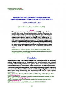
(a) (b) Fig. 1. (a) Schematic diagram of a single phase single energy source microgrid, (b) Closed-loop voltage control strategy of single phase single energy source microgrid.

the robustness of proposed algorithm against a set of uncertainties and loads. Remaining of this paper is organised as follows: Section II represents the islanded microgrid model, Section III describes the controller design. In Section IV, the performance of the controller is evaluated and V presents the conclusion.

principle with τ  [−1, 1]. This control loop needs high bandwidth with accurate duty ratio τ for high voltage tracking performance.

II. MODELLING OF THE ISLANDED MICROGRID

iL = iC + ig

2.1. Microgrid configuration Microgrid consists of loads, distributed generations, electrical energy storage (EES) and has an AC transmission system. The general microgrid layout is shown in Fig. 1(a). A voltage source inverter (VSI)is used between microgrid and DC energy source. The VSI is used to transport power from DC-side to ACside. As a VSI, an IGBT is used. The switching action of IGBT is represented as Vsw = τ Vdc , where τ is the duty ratio i.e. τ  [−1, 1] and Vdc represents the DC voltage source. An LC filter is also used at the AC-side of the VSI to reduce the switching ripple. During the steady state the average AC power Pac is equal to the DC power Pdc . 2.2. Voltage control In microgrid system, the desired grid voltage is tracked by the voltage control loop. The block diagram of the voltage control for microgrid is shown in Fig. 1(b). An IGBT is used as an VSI. From this figure, the closed loop grid voltage Vg is compared with the desired reference voltage of the microgrid in the voltage controller which produces error. Then the resultant voltage from the voltage controller determines the duty ratio τ for VSI using pulse width modulation (PWM)

2.3. Modeling of single phase microgrid From Fig. 1(a), the inductor current iL is given by the following equation: (1)

where, iC and ig are the capacitor and grid current respectfully. The controller scheme is based on: L

diL (t) = Vsw − Vg (t) dt

(2)

The switching voltage Vsw over a pulse width modulation (PWM) is given by: Vsw = τ Vdc

(3)

dVg = Ic dt

(4)

For grid voltage Vg : C

From (2) and (4), the derived state-space model is: dx = Ax + Bu dt

(5)

y = Cx + Du

(6)

Here, x is the state vector and u is the input vector of the microgrid system and d is the disturbances which is next to the state and input vector. These disturbances results in grid current because the micogrid structure is unknown for controlling tuning and changeable when loads or generators turn on and off.



     iL ; u = Vsw ; d = dˆ = ig Vg The state space is as follows:      1   iL 0 − L1 d iL = 1 + L Vsw + dt V Vg 0 0 C  g 0   ig − C1 The output of the system is         iL y = Vg = 0 1 Vg

subject to  APˆ + Pˆ AT + BY + Y T B T  Pˆ Y

x=

xT (0)Pˆ −1 x(0) ≤ γ

3.1. LQR-LMI framework for PID controller This section represents the concept of linear quadratic regulator (LQR) and linear matrix inequality (LMI) as a base for the design of robust PID controller. As the LQR control theory has a significant robustness [21], in several control problems the design of the controller is based on LQR control theory. Now consider a linear time invariant (LTI) system:

0

for any initial state x(0), where Q = QT ≥ 0 and R = RT > 0, i.e. Q and R are symmetric positive semi-definite matrix and symmetric positive √definite matrix, respectfully. Letting that (A, B) and ( Q, A) are controllable and observable respectfully. Then the optimal control minimising J is given by the linear state feedback law [21]: u∗ = −Kx = −R−1 B T P x where P is the unique positive definite solution of the Algebraic Riccati Equation (ARE): A P + P A − P BR

−1

T

B P +Q=0

(9)

and the minimum quadratic cost is given by: Jmin = xT (0)P x(0)

(10)

Solving of ARE (9) is most important for the solution of LQR problem. By applying LMI technique, the LQR problem can be rewritten as an optimization problem over Pˆ and Y [20]: min xT (0)Pˆ −1 x(0) Pˆ ,Y

(13)

where γ is the specified upper bound. The above inequality can also be written as LMI:   γ xT (0) ≤ 0, Pˆ > 0 (14) xT (0) Pˆ So the optimization problem in (11) and (12) is converted to find a solution (P ∗ , Y ∗ ) which satisfies a set of LMIs in (12) and (14). For this the state feedback gain is given by K = −Y ∗ (P ∗ )−1

(15)

(7)

where u is the control signal, which minimize the quadratic cost: Z ∞ J(u) = (xT Qx + uT Ru)dt (8)

T

 YT 0  ≤ 0, −R−1 (12)

Pˆ > 0 where Y = −K Pˆ and Pˆ = P −1 . In many cases equation (11) is rewritten as:

III. ROBUST PID CONTROLLER DESIGN

x˙ = Ax + Bu; y = Cx + Du

Pˆ −Q−1 0

(11)

But in practice the system matrix [A, B] is not precisely known. Assume that [A, B] is uncertain but lies in a polytopic set: Ω = Cov{[A1 , B1 ], [A2 , B2 ], [A3 , B3 ], ..., [ANm , BNm ]} (16) where Cov refers to [A, B]  Ω if [A, B] =

Nm X

wi (x, u)[Ai , Bi ]

(17)

i=1

where Nm refers to the number of multiple models and wi refers the weighting functions constrained between 0 and 1 and satisfy Nm X

x, u = 1, f(x, u)  RNx × RNu

i=1

normally, LMIs in (12) and (14) are used to find solutions over all uncertain system Ω. But it is a challenging task. However due to the characteristics of polytopic systems, finding a solution only at the polytopic vertices is enough instead of all points within the polytopic. 3.2. Design of PID controller This section presents the design of PID controller for microgrid system using LMI based approach. The

D(s) R(s) +

E(s) -

PID controller

+

+ U(s)

Plant



Y(s)

 

Fig. 2. Block diagram of closed loop system with PID controller.

microgrid system presented in (5) and (6) is a second order system. The design of the controller is presented for second order system. The block diagram of the closed-loop system is shown in Fig. 2. Assume an uncertain second order system: q2 T (s) = 2 (18) s + p1 s + p2 where the parameters p1 , p2 and q2 vary in an interval: p1  [p1 , p1 ], p2  [p2 , p2 ], q2  [q2 , q2 ]

(19)

where pi , pi and qi , qi are lower and upper bounds for denominator and numerator of the system respectfully. The structure of a PID controller is as follows: Ki P1 (s) = Kp + + Kd (20) s Or, s2 Kd + sKp + Ki P1 (s) = (21) s Where Kp , Ki and Kd are the proportional gain, integral gain and derivative gain, respectfully. The proportional gain (Kp ) decreases the rise time, the integral gain (Ki ) decreases the steady state error but increases overshoot and derivative gain (Kd ) decreases overshoot and settling time. The aim of PID controller design is to find the specific PID settings for meeting the numerous design specifications. The state-space model of the feedback system can be expressed as: dx = Ax + Bu + Br, dt u = −Kx + Kp r + Kd r, ˙

(22)

y = Cx

where y is the output of the system, x is the state i.e.  T x = x1 x2 x3 and r the reference input, and 

0 A = −p2 1

1 −p1 0

     0 0 0 0 , B = q2  , Br =  0  0 0 −1 (23)

Fig. 3. H(α, ρ, φ) region.

 C= 1

0

  0 K = Kp

Kd

Ki



Here the PID controller design becomes a static state feedback controller and the feedback gain K holds the parameters of the PID controller. There are three uncertain parameters in (18) and (23). Also the polytopic uncertain set in (16) reduces to : Ω = Cov{[A1 , B1 ], [A2 , B2 ], [A3 , B3 , ..., [A8 , B8 ]} (24) where the vertex matrix [Ai , Bi ] are determined based on the system identification results.

3.3. LMI formation of pole-placement for robust PID controller This section represents the pole placement [23] in the left-half plane and LMI-based characterisation of pole regions. The extended Lyapunov theorem for this regions is also discussed here. It is known that the location of poles [24] affects on the transient response of a linear system. If ϕ = −ζωn ± jωd be the poles of a second order system, then the step response is characterised in the form of ωn = |ϕ|, ζ and ωd where ωn = |ϕ|, ζ and ωd are the undamped natural frequency, damping ratio and damped natural frequency respectfully. To get a satisfactory transient response, ϕ must lie in a desired region. For this, specific bounds can be put on ϕ. The desired regions are α-stability regions Re (s) ≤ −α, vertical strips, conic sectors etc. Fig. 3 shows a set of region H(α, ρ, φ) of complex numbers x + jy such as x < −α < 0, |x + jy| < ρ, tan φx < −|y|

(25)

This region of poles ensures a minimum decay rate α, a minimum damping ratio ζ = cos φ and a maximum undamped natural frequency ωd = ρ sin φ. In other

words, this region bounds the maximum frequency of oscillation, maximum overshoot, delay time, settling time and rise time [24]. In the next section the existing Laypunov condition for pole clustering subregions of the complex plane is reviewed. After this, the notation of LMI region and extent of the class of LMI regions for the design of robust PID controller is introduced.

represented by an LMI in z and z , or an LMI in x = Re(z) and y = Im(z). This states that the LMI regions are convex. Also for any z  L and fL (z) = fL (z) < 0, these LMI region are symmetric with respect to real axis. According to the Gutman’s theorem for LMI regions, there exists a m × m block matrix

3.3.1. Lyapunov conditions for pole

= [αki P + βki AP + βik P AT ]1≤k,i≤m (31) which characterised the pole location in a given LMI region. Where ⊗ denotes the Kronecker product matrices and ML = [µk i]1 ≤ k, i ≤ m is a m × m matrix [25]. Theorem 3.2: Matrix A is L-stable if there exists a symmetric matrix P such that

A dynamic system x˙ = Ax is called L stable if all the eigenvalues of matrix A lie in L, where L is a subregion of the complex left-half plane. Moreover, A is stable if there exists a symmetric matrix P satisfying AP + P AT < 0, P > 0.

(26)

But Gutman has extended this Lyapunov stability characterisation in different regions [22]. This regions are polynomial regions of the form: X (27) L = {z  C : cki z k z i < 0} 0≤k,i≤m

where cki = cik and are real. But this polynomial regions are not totally general and the region H(α, ρ, φ) in (25) cannot be represented in this form. Gutman’s fundamental result provides the polynomial regions in the form [22] of X cki Ak P (AT )i , P > 0 (28) k,i

where A is L stable if P is exist as a symmetric matrix. But Gutman’s characterization for controller design is complex due to polynomial nature of (28) and turning (28) into an LMI is probably impossible in systematic way. Hereafter, an alternative L-stability region is necessary for LMI-based representation. 3.3.2. LMI regions Definition 3.1: LMI region is defined as a subset L of complex plane if there exists a symmetric matrix α = [αki ]  Rm×m and a matrix β = [βki ]  Rm×m such that L = z  C : fL (z) < 0 (29)

ML (A, P ) := α ⊗ P + β ⊗ (AP ) + β T ⊗ (AP )T

ML (A, P ) < 0, P > 0.

(32)

Proof: see the Appendix [26]. But the substitution (P, AP, P AT ) ←→ (1, z, z T ) relates ML (A, P ) in (31) and fL (z) in (30). The disk radius ρ and center (−q, 0) is an LMI region if the LMI region is defined by the disk radius ρ and center (−q, 0) with characteristic function fL ), where   −ρ q + z (33) fL (z) = q + z −ρP In this case, (32) becomes   −ρP qP + AP ,P > 0 qP + P AT −ρP

(34)

Now take α = ρ = 0 in H(α, ρ, φ). It has been shown [27] that all the eigenvalues of A lie in H(0, 0, φ) if and only if there exist a positive definite matrix P such that (W ⊗ A)P + P (W ⊗ A)T < 0   sin φ cos φ where W = − cos φ − sin φ But   sin φ(z + z) sin φ(z − z) fφ (z) = cos φ(z − z) sin φ(z + z)

(35)

(36)

with fL (z) := α + zβ + zβ T = [αki + βki z + βik z]1≤k,i≤m (30) where the characteristic function fL takes values from m × m Hermitian matrices. In other view points, the subset of a complex plane is an LMI region and it is

is the characteristic function of the LMI region H(0, 0, φ). Theorem (3) results that the poles of A lie on H(0, 0, φ) if and only if there exists P > 0 such that   sin φ(AP + P AT ) sin φ(AP − P AT ) < 0 (37) cos φ(P AT − AP ) sin φ(AP + P AT )

or

Start

(W ⊗ A)Diag(P, P ) + Diag(P, P )(W ⊗ A)T < 0 (38) This last equations gives better structural information of P , which is better from an LMI optimization.

Theorem 3.2 provides the needs for a characterisation of stability region which is affine in the A matrix. In contrast, theorem 3.2 provides that the close loop poles of a system with a state feedback u = Kx are lie in the region H(α, ρ, φ) if and only if there exists a symmetric positive definite matrix P and a matrix Y such that [26]



−ρP AP + BY

cos φ(AP + P AT +  BY + Y T B T )  sin φ(−AP + P AT − BY + Y T B T )

 P AT + Y T B T