Load Balanced Mapping of Distributed Objects to ... - Semantic Scholar

JOURNAL OF PARALLEL AND DISTRIBUTED COMPUTING ARTICLE NO.

34, 117–136 (1996)

0050

Load Balanced Mapping of Distributed Objects to Minimize Network Communication ALEXANDER D. STOYENKO,*,1 JAN BOSCH,†,2 MEHMET AKS¸IT,‡,3 AND THOMAS J. MARLOWE*,¶,4 *Real-Time Computing Laboratory, Department of Computer and Information Science, New Jersey Institute of Technology, University Heights, Newark, New Jersey 07102; †University of Karlskrona/Ronneby, Department of Computer Science and Economics, Ronneby, Sweden; ‡Department of Computer Science, University of Twente, P.O. Box 217, 7500 AE Enschede, the Netherlands; and ¶Department of Mathematics and Computer Science, Seton Hall University, South Orange, New Jersey 07079

This paper introduces a new load balancing and communication minimizing heuristic used in the Inverse Remote Procedure Call (IRPC) system. While the paper briefly describes the IRPC system, the focus is on the new IRPC assignment heuristic. The IRPC compiler maps a distributed program to a graph that represents program objects and their dependencies (due to invocations and parameter passing) as nodes and edges, respectively. In the graph, the system preserves conditional and iterative flows, records network transmission and execution costs, and marks nodes that have to reside at specific network sites. The graph is then partitioned by the heuristic to derive a (sub)optimal node assignment to network sites minimizing load balancing and network data transport. The resulting program partition is then reflected in the physical object distribution, and remote and local object communication is transparently implemented. The compiler and run-time system use efficient implementation techniques such as type prediction, inlining, splitting and subprogram passing. The last of these allows remote code to be copied to local data, as an alternative to copying data to the remote site, whenever this will reduce network data transport. The IRPC graph partitioning heuristic operates in time O(E(log d 1 l 1 log M )), where M is the number of network sites, E is the number of communication edges, and d is the maximum degree of a node; l is a parameter of the algorithm, and can vary between 1 and N, where N is the number of communicating objects. This complexity is more nearly independent of M, and considerably better in terms of E and N, than that of previously known related algorithms, such as A*, which employs backtracking and is potentially exponential, or the max-flow/min-cut class of network flow algorithms or heuristics which tend to be at least of V(MN2E), and it can be made (by choosing l appropriately) as efficient as even such fast heuristics as heaviest-edge-first, minimal communication, and Kernighan–Lin. In an extensive quantitative evaluation, the heuristic has been demonstrated to perform very well, giving on the average 75% traffic cost reductions for over 95% of the programs when compared to random partitioning, and outperforming in cost reduction and actual execution time the three aforementioned fast heuristics, even with a 1

E-mail: E-mail: 3 E-mail: 4 E-mail: 2

[email protected]. [email protected]. [email protected]. [email protected].

large l. Thus, to the best of our knowledge, this is the first report of a well-performing assignment heuristic that is both essentially linear in the number of communication edges, and better than existing, established heuristics of no better complexity.  1996 Academic Press, Inc.

1. INTRODUCTION

The use of distributed software and hardware architectures is widespread and accelerating. In order to utilize a distributed architecture fully, software engineers need to develop cooperating software modules running on different machines. One well-known approach to constructing distributed applications is through the use of remote procedure calls (RPC’s). The RPC model is based on the socalled client–server paradigm, and is similar to local procedure calling. A major difference from the local call is that an RPC allows a program to call procedures on a different computer or in a different address space on the same computer. The call is sent in the form of a request message to a remote server process, which sends back a reply message to the client. In contrast to local procedures, remote procedures cannot share the client program’s address space, and as a result, input and output parameters have to be copied between processes. The RPC construct is simple and powerful because it provides a transparent remote calling mechanism which is semantically similar or identical to the traditional local call mechanism. A great many distributed computer applications have substantial computation and network communication requirements. For instance, a number of hardware and software vendors have recently announced strategic commitments to multimedia computing—a distributed application area well known for its use of CPU-intensive algorithms and bulky data for representation, manipulation, and transmission of images, voice, and video [1]. Distributed multimedia systems can be considered a natural extension of today’s distributed systems. Typical examples are computer-supported education, desktop multimedia processing, office and hospital information systems, information kiosks, point of repair, browse, and sell, and entertain-

117 0743-7315/96 $18.00 Copyright  1996 by Academic Press, Inc. All rights of reproduction in any form reserved.

118

STOYENKO ET AL.

ment. Some multimedia applications require dedicated server machines, such as audio and video recorders/composers, to be shared by different application components. Most RPC mechanisms would encounter serious performance problems in dealing with such distributed applications, due to the unbalanced computation task assignments and bulky data copying between machines. One possible solution to these performance problems is to provide more sophisticated call and task assignment mechanisms to the programmer so that he or she can balance the computation load while optimizing remote calls. This approach, however, has a significant drawback in that it requires the programmer both to deal with complex computation and communication semantics which are very different from the familiar programming model, and to become an overall performance expert in his or her system. We believe that the programmer should not be confronted with the details of distribution, task assignment, and communication and their costs, but that instead, transparent and automatic mechanisms must be provided. One aspect of distributed systems is the distribution of program modules, to balance workload and minimize interprocessor communication. Distribution of program modules is a form of graph partitioning, whose optimal solution finding is NP-complete. To address this problem, we introduce a new accurate, linear heuristic algorithm called the Inverse Remote Procedure Calls (IRPC’s) heuristic, which generates a (sub)optimal task-to-processor assignment subject to simultaneous execution load balancing and communication cost minimization. The system is called inverse because it frequently (1) moves procedure code transparently to the site of the caller (subprogram passing), where the original program would have copied bulky data objects to the called procedure site, or (2) when procedures are grouped in objects, invokes methods of the calling object from the method/procedure at the called site, which may make access to caller data more efficient. The IRPC system also provides complete compile- and run-time support for transparent program distribution and interconnection. As our approach is based on objectoriented concepts, the IRPC compiler and run-time system support employ such techniques as type prediction, inlining, method splitting, and subprogram passing. Moreover, the system provides language-level stubs for all run-time distributed calling and communication. While many aspects of IRPC—a system which incorporates not only a heuristic task assignment algorithm but also a compiler, a stub generator, and a run-time system—are new, in this paper we focus on the task assignment heuristic. We have tested the heuristic for a large set of randomly generated and randomly assigned application programs.5 The IRPC heuristic has performed quite well, finding better distributions for over 95% of the programs and decreasing RPC transmission costs on the overall average of 75%.

The heuristic has complexity O(E(log d 1 l 1 log M ), where M is the number of network sites, E the number of communication edges, and d the maximum degree of a node; l is a parameter of the algorithm, and can vary between 1 and N, where N is the number of communicating objects. This complexity is largely independent of M, and the algorithm as a whole is substantially better in terms of overall complexity than related algorithms and heuristics. We have also tested the heuristic against three wellestablished, ‘‘classic’’ heuristics, namely, heaviest-edgefirst, minimal communication, and Kernighan–Lin, of respective complexity at least V(E log E), V(M E), and V(N 2E /M ) (see [24]). As Section 5 shows, the IRPC heuristic clearly outperforms these other heuristics in practice, both in terms of quality of solution and actual solution cost. This paper is organized as follows. In Section 2 we discuss background and related work. Section 3 briefly presents the language and system model. Section 3 details program graph construction. The IRPC heuristic migrates program objects by partitioning the corresponding program graph, aiming to balance the execution load while minimizing network communications. The partitioning is developed, presented, and evaluated qualitatively in Section 4. In Section 5 a detailed, extensive quantitative evaluation of the IRPC heuristic is reported. Section 6 summarizes our findings and gives directions for further research. 2. BACKGROUND AND RELATED WORK

Our work on the IRPC heuristic is related to graph partitioning algorithms and to resource allocation and migration algorithms. In what follows we discuss relevant background and related work in each of these topics.6

2.1. Graph Partitioning Algorithms Many practical problems, such as transportation, distribution, and communication systems, are designed and solved through graph models and graph partitioning algorithms, as summarized, for example, in [32]. Network flow algorithms address finding the maximum possible flow in a network. Much work in these algorithms has concentrated on networks with a single source and a single sink node [35]. The seminal max-flow-min-cut algorithm and theorem of Ford and Fulkerson [10] was followed by the first polynomial-time optimal algorithm (of O(E 2N ), where E and N are the numbers of edges and nodes, respectively) by Edmonds and Karp [9]. Improved polynomialtime optimal algorithms followed, among these [5, 7, 11, 12, 17]. Such algorithms’ complexities have remained worse than O(EN ), however; in fact, any practical algorithm tends to have complexity close to O(EN 2). In real programs, E tends to grow only slightly faster than linearly in N, although one can exhibit families even of structured 6

5

While the programs have been generated randomly, the generation parameters have been adapted from a real multi-media distributed system.

The IRPC project in general is related to works in remote procedure calls (RPCs) and some object-oriented systems. A discussion of related work in these two areas can be found in [23].

119

LOAD BALANCED MAPPING

programs for which E is V(N 2). Thus, a practical optimal solution must be worse than order O(N 3), which we consider computationally prohibitive. Moreover, optimal network algorithms do not scale up well to networks with multiple sources and sinks, as these almost always make the problem NP-complete. One other efficient graph partitioning heuristic is due to Kernighan and Lin [13]. The heuristic essentially repeatedly picks a pair of sites and a pair of objects preassigned to each site and swaps those two objects whose exchange would decrease the cost at the site the most. The complexity of Kernighan–Lin is V(N 2E /M )), where M is the number of sites (processors), which is marginal for a practical algorithm. Other graph partitioning algorithms include backtracking, which in the worst case considers every partitioning possibility in an exponential, computationally prohibitive fashion, and the A* algorithm, which is a breadthfirst algorithm which starts by creating a number of partial solutions and then repeatedly advances the most promising one one step further. We originally considered the A* algorithm as promising for IRPC. Having implemented an adapted version of A* for code partitioning, however, we have observed, that the complexity of the algorithm depends heavily on the type of remote program. While in the rare best case A* performs well in polynomial time, in the average and worst cases, its complexity is exponential in the number of objects due to backtracking. We have therefore decided against the use of A*, and devised our own graph partitioning heuristics, of complexity essentially O(E log M ), as described in Section 4.

2.2. Resource Allocation and Migration Algorithms In the operating systems area, a considerable amount of work has been carried out in resource migration and allocation algorithms (compare [8]). In most cases, the problem is represented as a graph with (weighted) process nodes and (weighted) communication edges, and the optimal solution either is not decidable or is NP-complete [15]. Demand-based copying techniques have been used to reduce network data transfer. For example, Emerald [3] introduces a technique called call-by-move which transfers parameter objects only when they are referred to. In the so-called data shipping technique, used by several distributed file systems [18], data are delivered automatically to a process as they are needed. Caching algorithms enhance demand-based copying by using statistical information. Again, several distributed systems adopt caching schemes to reduce the average cost of data transmission [33]. A number of node techniques are actually fast heuristics, based on either random assignment or finding a local minimum. In random partitioning, nodes are allocated, at random, to any processor in which they will fit. In the heaviestedge-first algorithm, the nodes connected by the heaviest edges are allocated to the same processor. In the minimalremote-communication algorithm, processes are allocated in such a way that the total weight of the edges radiating

from each processor is minimized. Each unallocated process is tried on each processor, and is assigned to minimize the total weight of edges connected to nodes currently outside the processor. In the quantitative evaluation of the IRPC heuristic (see Section 5), we first assign nodes according to random partitioning and then re-assign using, in turn, four fast heuristics: the IRPC, the heaviest-edgefirst, the minimal-communication, and the Kernighan–Lin graph partitioning heuristics. Since the IRPC heuristic uses a combination execution–communication site cost measure, we actually enhanced the other three heuristics to use the same measure. Closely related to our work is processor task/module assignment, considering interprocessor communication costs and using network flow algorithms. In a seminal paper [19], Stone applies an optimal max-flow-min-cut algorithm (of the order of at least O(N 3)) to two-processor assignment, and suggests extensions to handle more than two processors. To the best of our knowledge, the most efficient among closely related contributions remain Lo’s O(MEN 2 log N ) (where M is the number of processors) heuristics for task assignment in distributed systems [16]. These have been shown to achieve optimal multiprocessor assignments in 22% of a large number of cases and practically never to produce a suboptimal assignment with cost more than 1.5 times worse than that of the optimal assignment. One important difference between our approach, on the one hand, and resource migration and allocation algorithms, on the other, is that we aim at a finer granularity, assigning objects or procedures to processors rather than entire processes. Consequently, in our applications the values of E and N tend to be very large, making the algorithms and heuristics described above prohibitively expensive. We thus seek, in the rest of the paper, a well-performing heuristic of order considerably better than V(N 3). 3. PROGRAMMING LANGUAGE AND COSTS OF DISTRIBUTION, COMMUNICATION, AND EXECUTION

3.1. The Language Model We assume that distributed programs are written in an object-oriented, distributed language, statically scoped and based on active persistent objects. The language does not support inheritance nor delegation, but incorporates an interface concept similar to that of Sina [2, 34]. An application consists of type declarations and an application description. Each type declaration contains internal objects, methods, an initializer, and a process. The application description declares all global objects and allows the programmer to declare environment dependencies of global objects; that is, objects dependent on processor resources are bound to machines which support those resources. The interface specifies exported methods for each object; calls to local methods or methods exported from subobjects use a object.method syntax with defaults.

120

STOYENKO ET AL.

Within a process or method, statements are executed sequentially. The number of active processes in the system is bounded from above by the number of objects in the system, as each object has its own process. For remote procedure calls, the process of the calling object is blocked and a new process is created at the called site to execute the requested method of the called object. After finishing method execution, the process dies and the return object, if available, is returned to the blocked calling process.

3.2. Deriving Distribution, Execution, and Communication Costs Given an application program, we make a number of assumptions on object distribution, communication, execution, and costs. Based on these assumptions, we compute these costs (on a per method, per process, and ultimately per object basis), consequently enabling the labeling of the nodes and the edges of the graph representation of the entire application (see 3). Internal Objects and State. Internal objects can be distributed, although access to internal objects must pass through the interface of the global object. However, only internal objects used as a parameter are distributable. It is the responsibility of any method invoked with an internal object parameter to make the relevant part of the object available at the site of the method. In addition, we assume that any site has enough storage to accommodate any number of objects. Operators. All operators are considered to be methods, whether primitive, user-defined, or available through libraries. The compiler and run-time system will make use of the distinction; the code of primitive methods is automatically available at all sites (and typically inlined), unlike that of user-defined and library methods. Library code will in general only be available on sites where the library or objects of the specific type are placed. Constants. Constants are provided by run-time support on every site, and the cost of manipulating constants is negligible. Thus, constants are never site-dependent, and never need to be transmitted over the network. Parameters. For every method invocation, the cost CP (where CP is a positive integer) of making a particular object P available at the method is known, via a special local cost estimate function, at the time of program partitioning.7 This cost only applies if P resides on a different site from the method, and is treated as zero otherwise. For convenience of program partitioning, the call to the cost estimate function—returning the cost of this single invocation—may be specified, as an optional directive ignored by the compiler. If the directive is omitted, the system provides a default value. Details can be found in [4, 22, 23]. 7 Including per call setup, messaging, switching, and routing—we have not yet addressed these and other types of communication overhead.

Invocation/Termination. The costs of directing a method of an object to execute and of returning a method termination acknowledgement are small although not negligible. For simplicity of presentation, we assume both costs to be an identical constant, C cost units, the size of the smallest network packet. Execution Cost—General. The compiler performs a schedulability analysis [27, 30] of each method and process to estimate the computation time the method/process will need. As an object is being compiled, the compiler builds a directed acyclic execution graph (DAG) for each method, unrolling loops, splitting and joining the graph where it finds conditionals, and providing placeholders where methods of other objects are called. The graphs representing these external methods are later inlined at the placeholders. As executable machine instructions are generated, the analyzer looks up their execution times in an executiontime table (which makes standard assumptions of predictable platform timing) and accumulates them in basic graph nodes, signifying straightline code executions. Execution Cost—Loops. The number of loop iterations significantly influences object/process execution time. Moreover, a loop may contain calls. To compare the costs of alternate assignments, it will be necessary to know the loop iteration count or bound. We assume that the count/ bound for a while-loop is estimated by yet another function, also available at partitioning time. For constant-count loops the function returns a constant value (naturally) and for others the function returns a profiled (or statistical) estimate. Recursion, wherever discovered, is treated in the same way as iteration. Execution Cost—Calls. A process can call three types of methods: methods of global objects other than the process’ own object, methods of internal objects, and methods of the process’ own object. The execution cost of a global method is added to the cost of the object owning the method. The execution cost of methods of an internal object is added to that internal object’s total if the internal object has added to the object itself. The execution cost of an object’s own methods is, naturally, added to the cost of the object itself, thus providing an estimate of the overall object execution time. A method, in turn, can call methods of global and internal objects only (but not methods of its own object), and these are handled similarly. Execution Cost—Contention. In conventional schedulability analysis, the DAGs of the methods are later used to determine contention among independently executing processes, through symbolic execution in the back end of the analyzer. However, for the purposes of guiding assignment, the IRPC and similar heuristics do not normally require such accurate contention estimates. In fact, we only accumulate execution times in the absence of contention.

121

LOAD BALANCED MAPPING

In cases where a conditional splits execution flow, we take the execution time to be the maximum of the two possible times. Constructing the Graph. A graph node represents a global object, or an internal object which is used as a parameter during execution. If the object is environment dependent, meaning that it has to reside at a particular network site, the node is labeled as such. Dependencies among objects are represented as graph edges. In our programs, two types of dependencies may be found. First, a direct invocation, in the body of a process P1 (or a method of an object O1), of a method of an object O2 constitutes a dependency of P1 (or O1) on O2 . Observe that indirect invocations do not constitute dependencies. Consider the following example: P1hO2?M1 (O4?M1(O6), O5) O3?M1(O7)j.8 In this example, a process P1 makes two calls. The first call is to the method M1 of object O2 , passing two parameters, namely (1) the method M1 of object O4 , passing this method in turn the object O6 as a parameter, and (2) the object O5 . The second call is to the method M1 of object O3 , passing in turn the object O7 as a parameter. Thus, P1 is dependent on O2 and O3 but not on O4 , O5 , O6 , or O7 . Second, if an object O1 is passed as a parameter to a method of an object O2 , then O2 is dependent on O1 . In our example, O2 is dependent on O4 and O5 , O4 is dependent on O6 , and O3 is dependent on O7 . We label graph nodes and edges with execution and communication costs, where per method, per process, and per object costs are derived—on the basis of compilerextracted information and calls to cost estimating functions—as discussed in [24]. Since a node represents a single object, its cost will be used as the node label. On the other hand, an edge label may represent the costs due to single or multiple calls; these costs will only be incurred if the two nodes incident on the edge are placed on different sites. The number of calls along a particular execution path is known since the code of every method and process has been unrolled. Communication costs (due to the parameters passed) are accumulated as straight sums where there is no conditional execution flow.9 Should an edge be representing a dependency discovered inside a branch of an ifstatement (and conditional flow thus be present), the edge is labeled with the triplet (C, IF, IF#), where the three elements of the triplet are respectively the edge cost, a flag indicating the branch of the if-statement (that is, the thenbranch or the else-branch), and a unique number distin-

guishing this if-statement from all others.10 Duplicate edges are unified, carrying the union of labels, with the sum of costs for each label. When two nodes are placed on different sites, all edges that make them adjacent are cut. In the resulting graph, the program is represented as a disjoint collection of connected subgraphs.11 (While the graph is derived using directed dependence edges, our subsequent analysis operates on the underlying undirected graph. This will result in better load-balancing as measured and projected during (re-)partitioning, although possibly in poor actual behavior on some call paths. With the addition of an outer loop to handle unreached nodes in a weakly connected component, the algorithm of Section 4 can be relatively easily adapted to work on the directed graph with no additional asymptotic complexity.) Since processes and objects are represented uniformly in the graph, we omit references to processes in the rest of the paper. There are no duplicate edges in the graph, though an edge may have more than one cost label (a straight cost and a triplet for each conditional branch the edge is involved in). The nodes corresponding to environment-dependent objects are labeled as such. Finally, we use the accumulated information to sort the edge lists by decreasing worst-case total cost. We first need to assign a definitive cost to each edge. Since the worstcase cost on an edge will correspond to the maximum on any execution path, which will correspond (with appropriate loop multipliers) to some set of nested conditionals. This set of conditionals, and its cost, can be found by taking maxima on branches in a bottom-up traversal of the conditional nesting tree: if conditional q is nested in the true branch of conditional p, we will add the maximum branch cost for q to the true branch cost for p, and so on. After this computation, sorting is direct. While the cost for this processing is O(E log d ), where d is the maximum degree of a node, this is a one-time cost. It depends only on the code of the program, and not on the topology, and does not need to be recomputed if the graph has to be repartitioned. 4. PARTITIONING THE GRAPH

Given a program graph, possibly with some environment-dependent nodes (that is, objects, such as resource managers, which must be assigned to specific processors), we need to partition the graph over available sites. Ideally, we would like to find a partitioning heuristic that balances the load evenly over the available processors and aims to

8

For clarity, we omit cost estimate functions in this example. The exact effect of unrolling is as follows. Should an edge represent a dependency discovered inside a while-loop, the cost of the edge is computed as the cost returned by the cost estimate function times the number returned by the number of iterations estimate function (of that loop). Should an edge represent a dependency due to a conditional expression in a while-loop, the cost of the edge is computed the estimated number of iterations plus one (and times C). Recursive calls are unrolled similarly. 9

10 A fourth component could be added for profiling information if available. We do not consider conditional profiling further in this paper. 11 It is possible to have a MAIN process of some kind, whose job it is to instantiate every other process at program start time. Then, there would be a dependency from every other process to the MAIN (and hence the entire graph would be connected, assuming every object has a purpose in the program). However, we do not insist on having such a MAIN.

122

STOYENKO ET AL.

minimize the sum of communication costs along the edges cut by the partition, and works considerably faster than time complexity V(N 3). The heuristic presented here bases its assignment decisions on (1) choosing the least loaded site for likely future assignments among all sites, and (2) choosing the edge which minimizes a combination load-balancing and communication-minimizing formula among all possible cut edges. We will see in the qualitative and quantitative evaluation Sections that the heuristic in fact works very fast and produces good results. We now present an outline of the heuristic. A detailed description and detailed complexity analysis can be found in [24], and summary complexity analysis in Appendix B. The fundamental approach in the heuristic is to enable quick partitioning by avoiding backtracking totally. Since there needs to be a cut between any two environmentdependent nodes at different sites, the heuristic always follows paths beginning with an environment-dependent node. The heuristic repeatedly attempts to find paths originating at an environment-dependent node and identifying cuts optimal to a subset of possible paths between that node and some other possible environment-dependent node (residing at a different site). Should the paths be disjoint, the cut will in fact be optimal. On the other hand, should the heuristic discover intersecting paths, it will do a cut before a third intersecting path can be found, in order to avoid backtracking. If the heuristic loops or hits a deadend or cycle without finding an environment-dependent node residing elsewhere, the loop, dead-end, or cycle is remembered, until either a path intersecting with it is found (necessitating a cut) or the heuristic runs out of possible paths, at which point all nodes in the loop, dead-end, or cycle are placed on the same site as the originating environment-dependent node. The heuristic proceeds as follows. Initially, all environment-dependent nodes are permanently assigned by environmental constraints to their respective sites, all other nodes are not assigned, and all edges are travelable. Should there be a site without an environment-dependent node, a random node is picked and assigned there.12 The heuristic repeatedly picks a permanently assigned node with at least one adjacent travelable edge from the site with least cost (where cost is the sum of execution of nodes currently assigned to the site and the communication cost of their associated cut edges). Having picked such a node, the heuristic develops as long a path originating at the node as possible, by repeatedly picking the most expensive travelable edge available. As nodes and edges are encountered, they are labeled: the nodes as temporarily assigned to the same site as the path-originating node, and the edges as non-travelable. For each path, construction stops when no 12 We assume that the number of nodes is relatively large compared to the number of sites. Thus, a random assignment of a single node where there are no environment-dependent nodes is very unlikely to destabilize the overall eventual assignment.

more travelable edges can be taken, or when a node already assigned to a site is encountered, or a maximum length l is attained. Figure 1 presents a number of possibilities for which the path cannot be developed further. These include running out of edges (a dead-end), hitting a node in the path being generated (temporarily assigned to the same site—a loop), a node permanently assigned to the same site (a cycle), a node permanently assigned to a different site (a normal path), or a node which is part of a previously developed path, or a dead-end, a loop, a cycle, or a normal path. This last case means that two intersecting paths have been discovered and cutting is required. A path of length l not in any of the above is called a partial path. In Fig. 1 and consequent figures that present various cases which the heuristic encounters, nodes from different sites are drawn in different planar shapes (e.g. triangles, squares and ovals) and permanently and temporarily assigned nodes are presented as solid- and dotted(broken)-outlined shapes, respectively. While cutting two intersecting paths is linear in terms of the total length, the same operation will require backtracking and is consequently NP-complete for three or more intersecting paths. Consequently, whenever two intersecting paths are discovered, they are cut right away. All nodes in the cut paths are assigned permanently to the appropriate site (possibly changing their previous temporary assignments), and the costs of the cut edges become the only relevant communication costs in the paths. Should a cut not be needed (this occurs when another independent, nonintersecting path is discovered or the heuristic runs out of edges to take), the path is remembered for future cutting. Cutting a path is based on load balancing and minimization of interprocessor communication, which, in principle, are two contradictory requirements. The cost of a site is defined as the sum of the execution (node) cost of all objects assigned to the site and the communication (cut edge) cost with objects (nodes) at other sites. The cut in a path between two sites S1 and S2 occurs on the edge

FIG. 1. Possible paths constructed by the heuristic.

123

LOAD BALANCED MAPPING

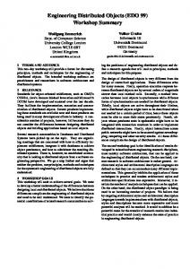
which minimizes the maximum of the costs of the two sites. This can be shown simultaneously to minimize the increase in the cost of the more expensive site and to maximize the decrease of the difference in the cost between S1 and S2 . All nodes at S1’s side of the cut edge are labeled S1 and all nodes at S2’s side are labeled S2 . In the case of two intersecting paths two or three sites may be involved. The heuristic first cuts the path between the two least costly sites (if there are only two sites, then the more expensive path is cut first), and only then the remaining path (connected to the most expensive site). Again, the rationale is to keep the site costs as balanced as possible while trying also to minimize communication costs. Whenever no nodes can be picked to develop new paths, the nodes temporarily assigned to the site with the least cost are assigned there permanently; this may of course change site cost and result in a different site becoming least cost, allowing different nodes to become enabled. (A partial path is expanded before assignment; assignment may still be required, but this may also result in a CUT, or in new nodes from which paths can be developed.) If still no conforming (meaning permanently assigned and adjacent to at least one travelable edge) nodes on the leastcost site can be found after this permanent assignment, the site with the next least cost is picked for the assignment, and so on, until either a node is made available for new path development or all nodes have been permanently assigned (and the heuristic thus terminates). The CUT TWO PATHS procedure is the central part of the heuristic. Called whenever two intersecting paths (obviously spanning at least two distinct sites) are discovered, the procedure works as follows. By construction, the nodes in the two paths can belong to at most three distinct sites (otherwise, either they would not have intersected or at least one path would already have been cut and permanently partitioned). In what follows, all cases and subcases are discussed, and furthermore, Figures are used to illustrate one representative subcase in each case (figures for the rest of the subcases are omitted for brevity). In all relevant figures (2 through 5), nodes are labeled with node numbers and execution costs in brackets, and edges are labeled with communication costs. Three Sites. Should the two paths span across three distinct sites (see Fig. 2), then clearly there are no partial paths, loops, cycles, or dead-ends, and exactly two cuts are required to partition (‘‘cutting off’’ one site from the two remaining, and then partitioning those two). The first cut is done between the two least expensive sites in an attempt to add more nodes to them, leaving fewer for the third site and resulting in an improved across-site balance. Observe that once a node has been permanently assigned, all edges from other nodes permanently assigned to it turn from directed to undirected. The reader may wish to verify for herself/himself that in considering where to make the first cut, possible cost pairs (circle,triangle) are (106,75),

FIG. 2. Three sites.

(101,84), (96,91), (90,93), and (90,107). For the second cut, the corresponding pairs (square,triangle) are (105,96), (98,100), (102,116). Of these, (90,93) and (98,100) are of course chosen, respectively. Observe how the maximum difference in costs among the three sites has been reduced from 17 to 10. Two Sites—First Discovered Path across Both. Should the two paths span across only two distinct sites, there are a number of cases to consider. If the first-discovered path spans across the two sites, then it is cut first. If the cut leaves the intersecting node in the site with the origin of the first path (see Fig. 3—the intersecting node is of course

FIG. 3. Two sites—first-discovered path across both (one case).

124

STOYENKO ET AL.

FIG. 4. Two sites—first-discovered path a dead-end, partial path, or cycle within one site (case of a dead-end).

node 4), then the nodes have been partitioned between the two sites. Otherwise, the other path is cut (and then the partitioning is for certain complete). There is a symmetric case, identically treated, where the concatenation of the second-discovered path and the subpath of the firstdiscovered path from the intersecting node on spans across the two sites. Two Sites—First Discovered Path a Partial Path, DeadEnd or a Cycle within One Site. Should the first-discovered path be contained within a single site, it must have been either a partial path, dead-end, a cycle, or a loop. If the path is a dead-end or partial path, a single cut is done between the two sites (along the path from the origin of the first path via the intersecting node on to the second path). After the cut, in the case of a dead-end, the subpath of the first path from the intersecting node on becomes a dead-end path at one of the two sites (the same site as that of the intersecting node); the rest of the nodes have now been partitioned permanently across the two sites (see Fig. 4—observe that even though the partitioning of the nodes in the two original paths is not quite complete yet, much progress has been made). For a partial path, the remaining portion of the first path is still partial (and assigned to one of the two sites), but no longer of maximum length; it is extended until it is of maximal length, or one of the other cases results, in which case the resulting path is labeled accordingly. If the path is a cycle, the same cut (as for the dead-end) is done. If after the cut the intersecting node stays at the site of the first path, then the first path’s subpath from this node on becomes a new cycle path. Otherwise, the direction of this subpath is reversed and the new path is normal (not a cycle, a dead-end or a loop, but rather starts at one site and ends at another). Two Sites—First-Discovered Path a Loop within One Site. If the first path is a loop, there are three cases to consider. If the intersecting node is strictly in the handle of the loop, then the concatenation of the handle up to

the node and the second path is cut. After the cut, the subpath of the first path from the intersection node on becomes a loop at the same site as the intersecting node (see Fig. 5—the intersecting node of course is node 2; observe, again, that while there is still work to do, much progress in assigning the nodes has taken place). If the intersecting node is at the knot of the loop (which is also the terminal of the first path), then the concatenation of the entire handle, the knot and the second path is cut. After the cut, the subpath of the first path from the intersection node on becomes a cycle at the same site as the intersecting node. Finally, if the intersecting node is strictly in the cycle originating at the knot (which is also the terminal of the first path), then the concatenation of the subpath of the first path from the origin through the intersecting node and the second path is cut. After the cut, if the knot and the intersecting node are at the same site, the subpath from the intersection node back to the intersection becomes a cycle at the same site. Otherwise, the subpath reverses its direction and becomes a normal path across the two sites (not a cycle, a loop, or a dead-end). Although the heuristic is suboptimal, we strongly believe that situations in which a poor node assignment is produced are rare. The belief is substantiated by the very encouraging results found in the extensive quantitative evaluation reported in Section 5. 5. EVALUATION

The performance of the IRPC heuristic has been tested extensively, on a large set of automatically-generated programs. The parameters for program generation have been based on those observed in a real distributed multimedia system at the University of Twente. There have been two tests, using the parameter l 5 N (that is, without partial paths). In both tests, for every program, its objects have been assigned randomly (and the overall costs for each site have been computed). In the first test we have assessed how the IRPC compares to three established heuristics: the minimal-communication, the heaviest-edge-first, and

FIG. 5. Two sites—first-discovered path a loop within one site (one case).

LOAD BALANCED MAPPING

the Kernighan–Lin. Specifically, given the random assignment, this same assignment has been improved, in turn, by applications of four heuristics, namely the IRPC and the three ‘‘competing’’ ones. In the second test we have assessed how various factors affect IRPC’s performance. Specifically, we have varied evaluation parameters, and have measured the IRPC’s improvement over the random assignment.

5.1. Testbed and Parameters As illustrated in Fig. 6, our testbed consists of four functional blocks: Parameter Input, Program Generator, Optimizer, and Measurement. The unit Parameter Input is used to control the input parameters of a particular test setting. The unit Program Generator accepts this input specification and generates a program which can be processed by a partitioning heuristics. The unit Optimizer transforms the program with respect to the heuristics. The unit Measurement gathers data from the original and optimized program code. In addition, the unit stores the collected data for a specified number of tests, and presents relevant characteristics in a structural way. The major input parameters are as follows:

• • • •

M is the number of network sites, SO represents parameters of objects, NO is the number of objects, DO is the percentage of environment-dependent objects on all M sites, • NS is the total number of statements, • TS is the description of types and proportional representations of various statements, and • NP is the number of programs generated in a test setting.

125

There are as many test settings—picked by the Program Generator—as there are combinations of the numbers of sites and the numbers of objects. Given a test setting, the Program Generator generates NP programs. For each program, the size and type of each object are determined, and then some objects are randomly chosen to be environment-dependent, and others assume random initial assignments on the M (with equal probability of 1/M of being assigned to any particular site) network sites. It is ensured that for every site at least one environment-dependent object is chosen. The program structure is as specified by the above parameters. Specifically, a random number generator adapted from the one published in [6] is used to guess the type or nesting depth of a particular statement. The generated numbers are normalized with respect to the value domain of the parameters. Consequently, minimum and maximum values of each parameter are also specified to the Program Generator. The parameter SO is a sextuple (S 1O , S 2O , P S1O , P S2O , EOmin , EOmax ). S 1O represents conventional data types and control information, and S 2O is used for large objects, such as video and audio. The percentage of occurrence of each object category is specified in P S1O and P S2O (where P S1O 1 P S2O 5 100%). The execution time of an object is considered to be related to the size of the object and is between EOmin and EOmax times the size of the object. The parameters NS and TS together determine the number and the proportional representation of all statements in the program. The parameter TS is actually a triple ( Pmsg , Tif , Twh ), where Pmsg is the percentage of simple message sends, and Tif and Twh represent if- and while-statements, respectively. The three types of statements are distributed uniformly—subject to proportional representation and nesting (see below)—throughout the program. Observe that this distribution defines sources of communication

FIG. 6. The functional block diagram of the IRPC test environment.

126

STOYENKO ET AL.

edges (for messages). Targets (i.e., objects other than the source object) of communication edges are picked randomly. Thus, complete program graphs are defined through this procedure. Tif is a sextuple (Pif , Pifth , Nifs , Pifn1 , Pifn2 , Pifn3 ), where Pif is the percentage of if-statements, Pifth is the percentage of if–then-statements within Pif , Nifsn is the number of statements within an if-statement, and Pifn1 , Pifn2 , and Pifn3 are the percentages of if-statement nesting depths of 1, 2, and 3, respectively. Here, Pifn1 1 Pifn2 1 Pifn3 5 100%. The percentage of if-then-else-statements within Pif is computed as Pifthel 5 100% 2 Pifth . Twh is a quintuple (Pwh , Nwh , Pwhn1 , Pwhn2 , Pwhn3), where Pwh is the percentage of while-statements, Nwh is a uniform range of the number of statements within a while-statement, and Pwhn1 , Pwhn2 and Pwhn3 are the percentages of while-statement nesting depths of 1, 2, and 3, respectively. Here, Pwhn1 1 Pwhn2 1 Pwhn3 5 100%. Since there are only three types of statements, the relation Pmsg 1 Pif 1 Pwh 5 100% holds for every program. For each test setting, the unit Measurement collects the following data: the number of sites, the number of objects, the number of statements, the average fan-in/fan out of objects, the average nesting of control statements, the time to execute the program, the cost of the original program,13 and the cost of the optimized program. In every test, the cost improvement has been computed as (Old Cost 2 New Cost)/Old Cost.

5.2. First Test: IRPC versus Other Heuristics In this test, the parameter settings have been as follows:

• M: M-min 5 M-max 5 10 • SO: S 1O-min 5 4 bytes, S 1O-max 5 4 Kbytes,

• • • •

•

PS 1O 5 80% S 2O-min 5 10 Kbytes, S 2O-max 5 1 Mbytes, PS 2O 5 20% EOmin 5 0, EOmax 5 10 NO: NO-min 5 100, NO-max 5 390, (varying by 10) DO 5 15 NS: NS-min 5 1 times the current number of objects, NS-max 5 3 times the current number of objects TS: Pmsg 5 90%, Pif 5 5%, Pifth 5 50%, Nifs-min 5 1, Nifs-max 5 5, Pifn1 5 70%, Pifn2 5 20%, Pifn3 5 10% Pwh 5 5%, Nwh-min 5 1, Nwh-max 5 9, Pwhn1 5 70%, Pwhn2 5 20%, Pwhn3 5 10% NP 5 900

Throughout the tests, the cost of invoking a method or returning a method termination acknowledgement (C) is 256 bytes (the size of the smallest transmittable network packet on the Unix network system used in the evaluation). Observe that there are 30 possible numbers of objects (100,

FIG. 7. The complexity (execution times, in milliseconds, logarithmic scale) of the four heuristics: (j) irpc, (h) heaviest edge, (r) minimal communication, (e) Kernighan–Lin.

110, ..., 390) and exactly one possible number of sites (10), thus resulting in 30 different test settings—with 900 programs generated for each, to a total of 27,000 programs altogether. The plots in the rest of the section apply to a single (‘‘average’’ over 900) program within a test setting. We have fitted most evaluation graphs (in this and the next Section) with straight lines to summarize the effect of the independent variable on the dependent one. The straight lines have been generated by a linear regression algorithm. We have implemented the three suggested alternate assignment heuristics—heaviest-edge-first, minimal-communication (as defined in [8]), and Kernighan–Lin (as defined in [13])—and have applied them to the exact same set of programs as we have the IRPC heuristic. Lower bounds on the complexity of the three heuristics are derived in Appendix A, namely, V(E log E), V(ME), and V(N 2E/M ), respectively. In contrast, recall that IRPC has complexity at least comparable to that of the others, O(E(log d 1 l 1 log M )), where M is the number of network sites, N is the number of communicating objects, E is the number of communication edges, and d is the maximum degree of a node; l is a parameter of the algorithm, and can vary between 1 and N. Thus theoretically (for suitable choices of l) IRPC has cost comparable to minimal-communication or heaviestedge-first, and much better than Kernighan–Lin. IRPC will also tend to be more robust in response to increases in the values of N, M or E/M than the other heuristics. The key issues we have addressed have been the execution complexity we have observed (Fig. 7 and 8 display the complexities on logarithmic and linear scales, respectively—we are using the logarithmic scale to elaborate how the IRPC compares with the other heuristics) and the cost improvement over the random assignment each heuristic has generated as a function of the number of objects (Fig. 10).14 Since the number of sites is kept constant, the num-

13

These two costs are the maximum site costs of, respectively, the randomly assigned program and the program reassigned from that random assignment according to the heuristic in question.

14 Recall that improvement is measured as the fraction (Old Cost 2 New Cost)/Old Cost.

LOAD BALANCED MAPPING

127

FIG. 8. The complexity (execution times, in milliseconds, linear scale) of the four heuristics: (j) irpc, (h) heaviest edge, (r) minimal communication, (e) Kernighan–Lin.

ber of sites has the ‘‘constant multiplier’’ effect in the complexity of the three ‘‘competing’’ heuristics. Thus, the effect of the number of sites on any of the three heuristics has not been evident even though their complexity depends on that qualitatively. Since the number of edges— representing message passing among objects—in a typical object-oriented program is typically closer to the number of objects than to the number of objects squared (the latter would suggest that most objects send messages to most other objects—hardly a good methodology for building programs), the execution complexity of heaviest-edge-first has been less than quadratic (though more than linear) in the number of objects. The constant number of sites, having been accounted for, the observed complexities of the four heuristics seem to correspond well to their qualitative counterparts. The execution complexity (measured in milliseconds) of IRPC and minimal-communication has been low-constant linear and practically identical (minimal-communication has in fact been somewhat better; see Fig. 9). Heaviest-edge-first has been somewhere between linear and quadratic, and

FIG. 9. A closer look at the complexities of IRPC (j) and minimal communication (h).

FIG. 10. The cost improvements (over the random assignment) of the four heuristics: (j) heaviest edge, (h) irpc, (r) minimal communication, (e) Kernighan–Lin.

Kernighan–Lin has been more than quadratic (apparently around O(N 2 log N )). As far as the cost improvement, IRPC has fared about as well as heaviest-edge-first. In fact, as the number of objects grows, there appears to be a trend for the improvement (for both heuristics) to grow over the random, and for IRPC to improve over heaviest-edge-first. On the other hand, the improvements of the other two heuristics over the random assignment have been considerably less than those of IRPC or heaviest-edge-first, and even seem to worsen slowly as the number of objects grows. One somewhat surprising observation is that Kernighan–Lin—the most expensive heuristic—performed so poorly. One plausible reason is that node and edge costs (corresponding to execution and communication costs) take on a large range of values, while the simulation in [13] dealt with assigning virtual memory pages in to real memory pages15 (approximately constant node costs, and not much communication). Figure 11 has a table of cost ranking—first through fourth, expressed as percentages, over all 27,000 programs (thus, for instance, the IRPC has placed first in approximately 0.453553% 3 27,000 or 12,246 cases) for the four heuristics. This ranking places IRPC head-to-head with heaviestedge-first, and very much ahead of the others. To derive the expected rank of a heuristic, we take the sum of the percentage fractions the heuristic has placed first, second, third, and fourth, weighted (multiplied) by 1, 2, 3, and 4, respectively. Then IRPC, heaviest-edge-first, minimalcommunication, and Kernighan–Lin have average ranks of 1.624269 P 1.6, 1.775469 P 1.8, 3.139207 P 3.1, and 3.461054 P 3.5, respectively. Observe that while IRPC and heaviest-edge-first improve similarly over the random assignment of programs of 230 and 380 objects, IRPC requires 35 and 85 milliseconds for the two assignments, respectively, while heaviest15

See [13, p. 291].

128

STOYENKO ET AL.

Rank

IRPC

Heaviest-edge

Min-comm

Kernighan–Lin

First Second Third Fourth

0.453553 0.503531 0.008006 0.034909

0.456838 0.393559 0.066899 0.082704

0.079072 0.088744 0.446089 0.386095

0.010536 0.014166 0.479006 0.496292

FIG. 11. A ranking of the four heuristics.

edge-first requires about 4,000 and 18,000 (or 114 and 212 times more!). Since IRPC has performed far better than two other ‘‘competitors’’ and about the same as the third, which has considerably worse complexity and performance, we believe the IRPC heuristic to be considerably better for our class of program assignment problems.

5.3. Second Test: The Effects of Various Factors on IRPC’s Performance While IRPC outperforms other heuristics, we have undertaken another test to determine what impact various factors—namely the number of objects, the average FanIn/Out at ED nodes, the execution cost component, the proportion of ED objects, the number of sites, and the number of objects per site—have on the heuristic’s performance. The parameters for this evaluation have been as follows:

• M: M-min 5 2, M-max 5 10 • SO: S 1O-min 5 4 bytes, S 1O-max 5 4 Kbytes,

• • • •

•

PS 1O 5 80% S 2O-min 5 10 Kbytes, S 2O-max 5 1 Mbytes, PS 2O 5 20% EOmin 5 0, EOmax 5 10 NO: NO-min 5 100, NO-max 5 490 (in increments of 10) DO 5 15 NS: NS-min 5 1 times the current number of objects, NS-max 5 3 times the current number of objects TS: Pmsg 5 90%, Pif 5 5%, Pifth 5 50%, Nifs-min 5 1, Nifs-max 5 5, Pifn1 5 70%, Pifn2 5 20%, Pifn3 5 10% Pwh 5 5%, Nwh-min 5 1, Nwh-max 5 9, Pwhn1 5 70%, Pwhn2 5 20%, Pwhn3 5 10% NP 5 2000

5.3.1. Influence of the Number of Objects We evaluate the performance of the IRPC heuristic versus the number of objects. This test differs from all others in that the number of sites M is kept constant at 10. The result of this test is illustrated in Fig. 12. The heuristic finds a better distribution for 95% of the programs, and reports an average improvement of 75%. In the case of the remaining 5% of the programs, the random initial distribution is better than the distribution found by the heuristic. The performance improvement found by the heuristic depends somewhat on the number of objects. As the number of objects increases, the performance does not seem to deteriorate and possibly even increases somewhat.

FIG. 12. Performance improvement versus the number of objects.

Figure 13 depicts the time complexity of the heuristic, approximated by a polynomial function which is linear in the number of objects (that is, O(NO)). The plotted times are actual clock values (of our platform) in milliseconds. This complexity is the same as that derived qualitatively in the Appendix B. The random variations in the graph are due to network contention and memory swapping. 5.3.2. Influence of the Average Fan-In/Out In the second test, we evaluate the performance of the heuristic versus the average fan-in/out (FIO). FIO is measured as the average number of edges connected to the environment-dependent objects in the graph representation of the program. The results of the test are depicted in Fig. 14, demonstrating a modest linear improvement with the growth in the FIO. Specifically, the x-axis represents the change in the average FIO, by 1 from 4 through 15.16 Other parameters, including the communication costs, are varied as before. Thus, the same test settings are used as before, but they are repeated first for FIO 5 4, then for FIO 5 5, and so on through FIO 5 15. One might expect the heuristic to perform less well when the average FIO (and consequently the number of alternative paths out of an ED node) grows, since the heuristic only considers one or two paths at a time. However, as the FIO grows, so does the number of edges connecting ED nodes directly (recall that these edges are cut right away). Moreover, graph connectivity also grows, and with it the relative effect of the communication cost component (as contrasted with the execution cost component) on the overall site costs. The following argument suggests why the heuristic will tend to perform better in this case. Since (1) execution costs are generated randomly and uniformly, and (2) the initial random node assignment tends to distribute nodes uniformly among sites, the initial random assignment is also likely to distribute the execution cost component of overall site costs in a fairly balanced way. Since the heuristic works fairly well, in the resulting heuristic assignment the execution costs are again going to be fairly balanced. 16

The actual growth in the FIO is achieved by adding program edges— through increasing the proportional representation Pmag of message statements—in the generation.

LOAD BALANCED MAPPING

129

FIG. 13. Time complexity (execution time in milliseconds) versus the number of objects.

Thus, the improvement in the execution cost component between the initial and the heuristic assignments is likely to be modest. On the other hand, while the cost of a cut edge in the initial assignment is likely to be the average edge cost, the cost of a cut edge in the heuristic assignment is likely to be below average edge cost. Thus, the improvement in the communication cost component between the initial and the heuristic assignments is likely to be significant. Since the proportional effect of the communication component grows with the FIO, so does then the overall improvement, that is the performance of the heuristic.

FIG. 14. Performance improvement versus the average fan-in/out of environment-dependent objects.

5.3.3. Influence of Execution Cost In Fig. 15 the performance of the heuristic is measured as the effect of the execution cost component on the overall site cost is increased. Specifically, the x-axis represents the change in the multiplier X (varying by 1 from 0 through 50) where the execution cost of an object is computed as X times a basic size of the object (picked randomly by the Program Generator). Other parameters, including the communication costs, are varied as before. Thus, the same test settings are used as before, but they are repeated first for X 5 0, then for X 5 1 and so on through X 5 50. Not surprisingly, as the proportional effect of execution

FIG. 15. Performance improvement versus execution cost.

130

STOYENKO ET AL.

costs increases, the improvement achieved by the heuristic over the random assignment decreases. The figure thus exhibits modest, linear deterioration in performance. 5.3.4. Influence of Environment-Dependent Objects In this test, we measure the effect of the percentage of environment dependent objects on the performance of the heuristic. We use the same parameter settings as before with the exception of DO , which we vary from 10% to 90%. The result of this test is shown in Fig. 16. The percentage of environment-dependent objects degrades the performance of the heuristic approximately linearly. This effect is expected, since the fewer objects the heuristic is allowed to move, the less optimization is likely.

FIG. 17. Performance improvement versus the number of network sites.

5.3.5. Influence of the Number of Network Sites With the exception of the first test, every test described so far has been run for every value of M between 2 and 10, inclusively. Figure 17 shows the relation between the number of sites and the average performance of the heuristic. The performance of the heuristic deteriorates slowly (and linearly) as the number of sites increases. This is hardly surprising, since as the number of sites grows, the number of possible average balanced site assignments drops (all sites are homogeneous and consequently all symmetric assignments are considered as the same assignment). (In the extreme case of No 5 M, the number of possible different assignments is exactly one.) Consequently, the opportunity for the heuristic to improve upon the initial assignment decreases as the number of sites grows. 5.3.6. Influence of the Number of Objects per Network Site In Fig. 18 the relation between the number of objects per site and the average performance is plotted (based on the same data and runs as the previous test). As the number

of objects per site grows, so does the performance of the heuristic, by the same argument as just presented in the previous test. 6. CONCLUSIONS AND FUTURE WORK

To shield the distributed program writer from the complex problem of minimization of expensive network traffic, transparent and automatic mechanisms are needed. The IRPC system provides such a mechanism. Given a distributed program (written in an object-oriented concurrent language), the IRPC system compiles it to a program graph. Program objects and their dependencies (due to invocations and parameter passing) are represented as nodes and edges, respectively. Care is taken to preserve conditional and iterative flows. Real and would be execution and network transmission costs are recorded as node and edge labels respectively, nodes that have to reside at specific network sites are marked as such, and other nodes are marked with their initial site assignments. Once constructed, the graph is partitioned by the IRPC heuristic for the purpose of finding a (sub)optimal (in the sense of load balancing and minimization of network data transport) node assignment to the network sites. The resulting graph is then used to drive the object assignment and transparent stub generation and run-time RPC support (not discussed in this paper which focuses on the IRPC heuristic) for the distributed program. The low complexity—both inherent and observed in a practical implementation—of the IRPC heuristic makes it possible to apply the heuristic in not only static but also dynamic partitionings.17 Thus, distributed implementations 17

FIG. 16. Performance improvement versus the percentage of environment-dependent objects.

Our evaluation has suggested that ‘‘classic’’ low polynomial complexity heurstics either underperform when contrasted with the IRPC heuristic (as is the case with Kernighan-Lin and minimial-communication) or keep up in performance but, unlike the IRPC heuristic, become prohibitively expensive in terms of execution time (as is the case with heaviest-edgefirst—indeed, for a well-sized realistic program, applying heaviest-edgefirst to re-partition at run-time would be very time-consuming).

LOAD BALANCED MAPPING

131

FIG. 18. Performance improvement versus the number of objects per site.

of dynamically bound, object-oriented languages, such as SmallTalk, C11, or Sina, may benefit by invoking the IRPC heuristic at run-time, possibly as often as new objects are instantiated or new bindings are made. One can try improving further on the IRPC heuristic’s dynamic partitioning applicability. For instance, while the heuristic focuses on execution–communication load balancing, it makes no attempt to minimize the number of migrations required in a dynamic repartitioning. One heuristic way to minimize the effect of migration would be to apply the IRPC to an updated part of the program only (to ensure that only a part of a program is considered, the rest may be labeled environment-dependent). A more systematic way would be, however, to extend the heuristic to consider migrations as some part of the cost of the new partition. The latter method, however, would almost certainly increase execution time complexity of the heuristic.18 The heuristic’s complexity is considerably better than that of previously known algorithms, such as the A*, which employs backtracking and is potentially exponential, or the max-flow-min-cut network flow algorithms and heuristics, which are O(MN 4), and many of which do not even scale up past M 5 2. Moreover, the complexity of the IRPC 18 This increase could in fact be quite significant. It may also be observed that none of the low-polynomial order ‘‘classic’’ heuristics, including the three we have compared the IRPC one against, attempt to minimize the number of migrations either.

heuristic is logarithmic in M, and thus cannot be bettered by any algorithm which considers site costs (and is thus at least linear in M ) in making assignments. In our extensive tests, the IRPC heuristic has outperformed—in both cost improvement and execution time— other ‘‘competing’’ heuristics, namely heaviest-edge-first, minimal-communication, and Kernighan–Lin. In absolute terms, the IRPC heuristic has performed remarkably well, achieving on the average 75% improvement (over random assignment) in execution load balancing and communication cost reduction, for over 95% of the programs. The heuristic is not only stable but the cost improvements seem to even grow somewhat as the number of objects, and especially the number of objects per site, grow. This means that the more loaded the distributed system is, the better the heuristic is likely to perform. As the average fan-in/ fan-out (FIO) increases, so does the performance of the IRPC heuristic. Thus, the more communication-intensive the distributed application is, the better the heuristic will perform. On the other hand, the more CPU-intensive the application is, the less well the heuristic will perform (though it will still improve very considerably over a random object assignment!). One immediate extension of this work is to put realistic limits on network site and link capacities. Specifically, rather than addressing the general load-balancing and communication cost minimization problem in a homogeneous, completely connected network, we would treat the network as a set of connected heterogeneous sites, where node assignment should be

132

STOYENKO ET AL.

driven by site- and link-packing heuristics. Another extension would incorporate realistic overhead costs, due to migration, processor switching, communication, buffering and so forth, into cost computation. Yet another extension would be to incorporate not only load-balancing type of criteria, but also other ones, such as parallelism and deadlines (we have begun such work [31] since the original submission of this paper). However, the theoretical complexity of the heuristic depends on a parameter l. Values between max(log d, log M ) and N 2 M can be expected to give different and not clearly predictably related actual performance. Experimentation is needed to determine reasonable values of l in terms of N, M, E, and d. So far we have not addressed how the functions that estimate costs and the number of loop iterations should be designed. The functions should return values according to sound metrics, which would in turn be dependent on statistical program studies and programming methodologies. Assuming better cost reductions may be achieved without a significant loss in complexity, it may be of interest to try developing better heuristics. One additional obvious direction to proceed is to find a heuristic for cutting over more than two paths with minimal or completely without backtracking. Finally, the IRPC system should be integrated into a practical distributed environment. This task may present fundamental challenges even for a well-designed environment, such as that of SmallTalk. Even more significantly, the technical, engineering challenge will be quite formida-

ble, since an evolved distributed system would have to be integrated with a new (language) specification component for environment dependencies, costs estimation, graph generation, partitioning and re-generation, and a user feedback interface.

APPENDIX A. PSEUDOCODE FOR THE THREE PARTITION ALGORITHMS

While the basic ideas of the three partition algorithms we have used to compare the new IRPC heuristic against are very well-known, it is conceivable that exact implementations of them will differ. Moreover, to make the comparison as fair as possible, we decided to use the inherent lower V bounds for these algorithms (against the upper O bound of the IRPC heuristic). For these reason, it is both unnecessary and possibly impossible to show as detailed an implementation of the three algorithms as that of our new IRPC heuristic—which of course is introduced by and thus must be detailed in this paper. Rather, we provide high-level pseudocode implementations, followed by optimistic (thus giving the three ‘‘competing’’ heuristics the benefit of the doubt) complexity estimates. Finally, we stress that while the site costs as used in various heuristics may be different from ours (which is the combination of execution and communication costs), in our implementation of these heuristics, wherever site costs are computed, for fairness, the same combination site cost is used as used in the IRPC heuristic evaluation.

HEAVIEST EDGE FIRST ALGORITHM. initialize site costs to 0 sort set of edges by cost while travelable edges left hEdge 5 heaviest unassigned edge in the program graph if both objects connected to hEdge have been assigned mark hEdge untravelable update site costs else if one of the objects connected to hEdge has been assigned assign the unassigned object to the same site mark hEdge untravelable else assign both objects connected to hEdge to the site with the lowest associated cost endif endwhile MINIMAL-COMMUNICATION COST ALGORITHM. for all objects O in the program graph for all sites S in the system calculate the sitecost increase when O is assigned to S endfor assign O to a site with the smallest cost increase endfor

LOAD BALANCED MAPPING

133

KERNIGHAN –LIN GRAPH PARTITIONING.19 make an initial assignment of objects to sites using a linear heuristic of choice compute initial communication costs mark all objects as unlocked initialize a list of pairs of objects to empty do for all sites Si for all sites Sj for k 5 0 to minimum (#object Si , #objects Sj ) for all free objects in Si for all free objects in Sj find the pair (Oia , Ojb) switching which decreases the sum of costs of Si and Sj the most if such a pair exists add (Oia , Ojb ) to the worklist of pairs lock Oia and Ojb endfor endfor endfor for all pairs in the pair worklist exchange the objects (Oia , Ojb ) unlock the objects Oia and Ojb endfor endfor endfor calculate total system cost while system cost decreases

Lower Bounds on Complexity of the Three Heuristics. The complexity of minimal-communication is transparently V(ME ), since no global data structures (beyond unordered lists of objects and sites, and edge lists for individual objects) are required. There are MN iterations of the inner loop, and each looks at incident edges and does a linear computation of minimum cost; the total number of edges considered for each site over all iterations is clearly E. The cost of heaviest-edge-first is dominated by the cost of sorting the initial edge list, V(E log E ). Remaining costs are O(E), except for the cost of maintaining the least-cost site, which is O(E log M ) using a heap. Initialization in Kernighan–Lin costs V(E). Even assuming that N/M objects, each with 2E/N incident edges, are assigned to each site will give a complexity of V(N 2E/M ) for each iteration of the outer loop (since incident edges will have to be examined to determine changes in cost); less uniform work distributions will not radically change the resulting complexity. Since at least one iteration of the outer loop is required, this is a lower bound on the cost of the heuristic. 19

A careful reader may notice that the formulation in [13] is iterative binary in the way it considers sites, while our algorithm examines each pair of sites in a nested iterative fashion. This issue is rather minor and bears no effect on this heuristics’ fundamental performance.

APPENDIX B. SUMMARY COMPLEXITY ANALYSIS OF THE HEURISTIC

We now present summary complexity analysis. Details can be found in [24]. The heuristic clearly always terminates, since it starts with a finite number of nodes and edges, labels some nodes permanently at every iteration, and terminates when all have been labeled permanently. It can also be shown that the heuristic always produces a complete and consistent cut. Observe that the operation and, consequently, the complexity of the heuristic depends on the number of sites only in maintaining the site data structures. These are initialized, and then changed only when a path terminates or a node is permanently assigned. All changes are constant cost, except for the maintenance of the two site heaps, which has a cost of O(log M ) per update. We arrive at the complexity through the following set of lemmas. 1. The initial data structures can be set up in time O(N 1 M 1 E log d 1 E log M 1 M log M) 5 O(E(log M 1 log d )) and assignment of the V environment-dependent nodes and random nodes for other sites takes at most O(EV 1

134

STOYENKO ET AL.

M ) 5 O(E), where EV is the number of edges incident on the nodes of V. 2. Each CUT operation results in permanent assignment at least one node. Thus, the number of CUT operations is O(N ). 3. New paths are created only when a travelable edge (from a labeled to an unlabeled node) is discovered, at which point its target will be labeled (by the path), or when a single path is created in a CUT. The number of total paths created in the first way is thus at most N 2 M, and so the total number is O(N ). 4. Initialization and reversal of paths have constant cost. 5. A site and a node at the site (to try developing a path) are picked no more than O(E) times. 6. When new paths are developed, each edge is looked at at most once and constant work is required for each edge, except to update temporary costs. The latter cost requires at most O(d ) constant-cost updates. For each partial path, a constant amount of extra work may be required. The total cost for (new and partial) path development is O(E 1 N ). 7. Processing a single node requires at most O(d ) operations of cost at most O (log M ). In fact, since a node will be assigned exactly once, and an edge will have its second end assigned exactly once, the total cost is at most O(E log M ). 8. Temporary costs will be updated the first time when a node is placed on a path, and when it is assigned to a site, and when a path is reassigned to a new site as part of a CUT. The first two of these result in at most O(N 2 M ) invocations. For the third case, notice that each node can be reassigned at most l times, since at least one node on the path (currently containing at most l nodes not permanently assigned) will be permanently assigned. Thus the total cost in this case is no more than O(El). 9. Outside of updating temporary costs and processing nodes, each CUT has cost over all invocations at most O(E ), since clearly no edge can be cut more than once. 10. All other steps of the algorithm contribute at most a constant amount of work per path, O(N ). Thus the total cost is O(E (log d 1 l 1 log M )). However, as we indicated above, we can expect M ! N; moreover, as has repeatedly been observed in the programming language literature, E is in practice usually approximately linear in N, and d approximately constant. Finally, since the O(El) work arises only from reassigning nodes to new paths at different sites; if, as we expect, there are very few paths giving rise to cycles, loops, or dead-ends, only reassignment of partial paths will contribute to this cost. Thus, for an appropriate choice of l, since there will be few partial paths, each moreover reassigned only a few times, we can expect to see behavior effectively linear in E log M, and close to linear in N log M, in practice. APPENDIX C. SUMMARY OF COMPLEXITIES

We have shown the complexities of the IRPC and three competing heuristics to be

Heuristic

Complexity

IRPC min-comm heaviest-edge Kernighan–Lin

O(E (log d 1 l 1 log M )) V(ME ) V(E log E ) V(N 2E/M )

where N is the number of objects, E is the number of communication edges, M is the number of sites, d is the maximum degree of a node (which is obviously dominated by N ), and l is a parameter of the IRPC technique which can be chosen to be between 1 and N. ACKNOWLEDGMENTS The authors are indebted for partial support of this work to NATO Collaborative Grant CRG-901077, U.S. ONR Grant N00014-92-J-1367, AT&T UEDP Grant 91-134, NJIT SBR Grant 421250, and the University of Twente, Faculty of Computer Science. Stoyenko’s research is also supported by the Naval Surface Warfare Center, Siemens Corporate Research, Honeywell, DEC, Bailey Controls, and the Center for Manufacturing Systems at NJIT. This work began when Stoyenko and Aks¸it were, as a Research Staff Member and a Visiting Professor, respectively, with IBM T.J. Watson Research. The authors are indebted to the anonymous referees for their excellent comments and recommendations. A fruitful discussion with Aaron Watters led to an improvement in an earlier draft of this paper. The authors are grateful to all members of the Real-Time Computing Lab at NJIT and the TRESE research group at the University of Twente for their support.

REFERENCES 1. Association for Computing Machinery. ‘‘SIGGRAPH ’91: 18th International Conference on Computer Graphics and Interactive Techniques, Las Vegas, Nevada, 1991. 2. Aks¸it, M., and Tripathi, A. Data abstraction mechanisms in Sina/ST. OOPSLA ’88 Conference Proceedings. 1988, pp. 267–275. 3. Black, A., Hutchinson, N., Jul, E., Levy, H., and Carter, L. Distribution and abstract types in Emerald. IEEE Trans. Software SE-13, 1, (Jan. 1987), 65–76. 4. Chambers, C., and Ungar, D. Making pure object-oriented languages practical. OOPSLA ’91 Conference Proceedings. Phoenix, AZ, 1991, pp. 1–15. 5. Cherkassky, B. V. Algorithm of construction of maximal flow in networks with complexity of O(V2E ) operations. In Mathematical methods for the solution of economical problems, Vol. 7. Akademiya Nauk USSR, 1977, pp. 117–126. 6. Cooper, D., and Clancy, M. Oh! Pascal. Norton, New York, 1982. 7. Dinic, E. A. Algorithm for solution of a problem of maximal flow in a network with power estimation. Soviet Math. Dokl. 11 (1970), 1277–1280. 8. Donnett, J. G., Starkey, M., and Skillicorn, D. B. Effective algorithms for partitioning distributed programs. Proceedings of the 7th Annual International Phoenix Conference on Computers and Communications. March 1988, pp. 363–368. 9. Edmonds, J., and Karp, R. M. Theoretical improvements in algorithmic efficiency for network flow problems. J. Assoc. Comput. Mach. 19, 2 (1972), 248–264. 10. Ford, L. R., and Fulkerson, D. R. Flows in Networks. Princeton Univ. Press, Princeton, NJ, 1956. 11. Galil, Z. A new algorithm for the maximal flow problem. Proceedings of the 19th IEEE Symposium on the Foundations of Computer Science. Ann Arbor, MI, 1978, pp. 231–245. 12. Karzanov, A. V. Determining the maximal flow in a network by the method of preflows. Soviet Math. Dok. 15 (1974), 434–437.

LOAD BALANCED MAPPING 13. Kernighan, B. W., and Lin, S. An efficient heuristic procedure for partitioning graphs. Bell System Technical J (1970) 291–307. 14. Kligerman, E., and Stoyenko, A. D. Real-time Euclid: A language for reliable real-time systems. IEEE Trans. Software Engrg. SE-12, 9 (Sept. 1986), 940–949. 15. Lo, V. M. Task assignment in distributed systems. Ph.D. dissertation, Department of Computer Science, University of Illinois, 1983. 16. Lo, V. M. Algorithms for task assignment in distributed systems. IEEE Trans. Comput. 37, 11 (Nov. 1988), 1385–1397. 17. Malhotra, V. M., Pramodh-Kumar, M., and Maheshwari, S. N. An O(V3) algorithm for finding maximum flows in networks. Inform. Process. Lett. 7 (1978), 277–278. 18. Satyanarayanan, M., et al. The ITC distributed file system: Principles and design. Proceedings of the 10th Symposium on Operating System Principles. 1985, pp. 35–50. 19. Stone, H. S. Multiprocessor scheduling with the aid of network flow algorithms. IEEE Trans. Software Engrg. SE-3, 1 (Jan. 1977), 85–93. 20. Stoyenko, A. D. A schedulability analyzer for real-time Euclid. Proceedings of the IEEE 1987 Real-Time Systems Symposium. 1987, 218–225. 21. Stoyenko, A. D. A real-time language with a schedulability analyzer. Ph.D. thesis, Department of Computer Science, University of Toronto, 1987. 22. Stoyenko, A. D. SUPRA-RPC: SUBprogram PaRAmeters in Remote Procedure Calls. SOFTWARE—Practice and Experience. 1994. A shorter, preliminary version available in Proceedings of the 3rd ACM/ IEEE Symposium on Parallel and Distributed Processing. Dallas, TX, 1991. 23. Stoyenko, A. D., Aks¸it, M., and Bosch J. A new heuristic for loadbalanced assignment of objects and minimized network communication in distributed programs implemented through inverse remote procedure calls. Informatica Memorandum Number 91-91, Computer Science, University of Twente, the Netherlands, 1991. 24. Stoyenko, A. D., Aks¸it, M., Bosch, J., and Marlowe, T. J. A detailed discussion of the inverse remote procedure call heuristic. Department of Computer and Information Science, Research Report, New Jersey Institute of Technology, Newark, 1995. 25. Stoyenko, A. D., and Halang, W. A. Analysing PEARL programs for timely executability and schedulability. Proceedings of Prozessrechensysteme ’91, Informatik-Fachberichte, No. 269. Springer-Verlag, Berlin/Heidelberg/New York/Tokyo, 1991, pp. 90–102. 26. Stoyenko, A. D., and Halang, W. A. High-integrity PEARL: A language for industrial real-time applications. IEEE Software (July 1993). A longer version is available as High-integrity PEARL and its schedulability analyzer: Transferring state-of-the-art real-time software technology from university laboratories to industry. Department of Computer and Information Science Technical Report CIS91-16, New Jersey Institute of Technology, 1991. 27. Stoyenko, A. D., Hamacher, V. C., and Holt, R. C. Schedulability analysis of hard-real-time programs. IEEE Trans. Software Engrg. 17, 8 (Aug. 1991). 28. Stoyenko, A. D., and Marlowe, T. J. Schedulability, program transformations and real-time programming. Joint IEEE and IFAC/IFIP Workshop on Real-Time Systems. Atlanta, GA, 1991, pp. 33–41; also in Real Time Programming. Pergamon Elmsford, NY, 1992, pp. 33–41. 29. Stoyenko, A. D., and Marlowe, T. J. Polynomial-time transformations and schedulability analysis of parallel real-time programs with restricted resource contention. Real-Time Systems 4, 4 (Nov. 1992), 307–329. 30. Stoyenko, A. D., Marlowe, T. J., Halang, W. A., and Younis, M. Enabling efficient schedulability analysis through conditional linking and program transformations. Control Engrg. Practice 1, 1 (Jan. 1993). 31. Stoyenko, A. D., Welch, L. R., Marlowe, T. J., Cheng, B.-C., and Ganesh, A. K. Performance prediction functions for real-time software components. Computer and Information Science Research Report CIS-93-12, New Jersey Institute of Technology, 1993. 32. Syslo, M. J., Deo, N., and Kowalik, J. S. Discrete Optimization Algorithms. Prentice–Hall, New York, 1983.

135

33. Terry, D. B. Caching hints in distributed systems. IEEE Trans. Software Engrg. SE-13, 1 (Jan. 1987), 48–54. 34. Tripathi, A., and Aks¸it, M. Communication, scheduling and resource management in Sina. J. Object-Oriented Programming (Dec. 1988), 24–41. 35. Wilf, H. S. Algorithms and Complexity, Prentice–Hall, Englewood Cliffs, NJ, 1986.

ALEXANDER D. STOYENKO received a doctorate in computer science from the University of Toronto in 1987. Subsequently, he joined IBM T. J. Watson Research Center as a research staff member. Since Fall 1990, he has been on faculty with the Department of Computer and Information Science at the New Jersey Institute of Technology, where he founded and leads the Real-Time Computing Laboratory—which currently has five regular and four visiting faculty and sixteen Ph.D. students—and where he is currently an associate professor. Dr. Stoyenko has also held visiting and consulting appointments at the University of Twente, IBM Zuerich Research Laboratory, Fern Universitaet Hagen, Technical University of Eindhoven, Stanford University, Wang Institute of Graduate Studies, the University of Toronto, the Bank of Montreal, and other organizations. His research interests are in real-time computing, distributed and parallel computing, engineering of complex computer systems, programming languages, compilers and tools, real-time imaging, biomedical computing, and software re-use and integration. He has pioneered the notions of schedulability analysis and schedulability analyzable programming languages. Dr. Stoyenko has published over 80 times in books, refereed journals, and conferences. He is Founding Chair of the IEEE Technical Committee on Complexity in Computing (formerly the Technical Segments Committee on Engineering of Complex Computer Systems), and also of the annual IEEE Conference on Engineering of Complex Computer Systems. He served as Co-Director of the first NATO Advanced Study Institute on Real-Time Computing and served as Chair of a number of IEEE Workshops. Dr. Stoyenko is the Founding CoEditor-in-Chief (with Dr. Phil Laplante) of the journal Real-Time Imaging. He was the keynote speaker at the PEARL’90 and IFAC WRTP’94 conferences, is an associate editor of the journal Control Engineering Practice, has been Guest Editor of the journal Real-Time Systems and of the Journal of Electronic Imaging, and is an invited member of the IFAC TC on Computers Working Group on Real-Time Programming, the U.S. Navy Software Specification and Synthesis Working Group, and a Senior Member of the IEEE. His professional activities have been supported by grants from NATO, ONR, NSWC, NSF, ARPA, AT& T, AT&T Foundation, Siemens Corporate Research, DEC, Bellcore, Honeywell, Bailey Control Systems, the Center for Manufacturing Systems at NJIT, and the State of New Jersey. MEHMET AKSIT holds an M.Sc. from the Technical University of Eindhoven and a Ph.D. from the University of Twente. Currently, he is working as an associate professor at the University of Twente. He is the leader of the Twente Research and Education on Software Engineering (TRESE) project. He visited the IBM Thomas J. Watson Research Center from September to December 1989. He is the principle inventor of objectcomposition-filters, atomic delegations, associative inheritance and delegation mechanisms, abstract communication types, and fuzzy-logic based object-oriented methods and metrics. He has identified and defined a set of new problems related to object-oriented analysis and design. His areas of interests are object-oriented analysis and design of distributed software systems, object-oriented CASE tools, and programming environments, languages, and methods. JAN BOSCH received an M.Sc. in computer science from the University of Twente, the Netherlands, in 1991 and a Ph.D. in computer science from Lund University, Sweden, in 1995. Currently, he is an assistant professor at the University of Karlskrona/Ronneby, Sweden. His research interests include extensible object-oriented language models, paradigm extensibility, object-oriented compilation techniques, and object-oriented software architectures.

136

STOYENKO ET AL.

THOMAS J. MARLOWE is Professor of Mathematics and Computer Science at Seton Hall University and a Visiting Research Professor at New Jersey Institute of Technology and at Rutgers University. Dr. Marlowe received his B.S. in mathematics at Seton Hall University in 1970, and holds Ph.D.’s in mathematics (1975) and computer science (1989) from Rutgers University. His research interests include compilers and compiler Received June 21, 1993; revised April 28, 1995; accepted October 30, 1995

optimization, particularly the theory of data flow analysis; language and compiler support for real-time and complex systems; engineering of multiobjective complex computer systems; and algorithmic graph theory. He has collaborated on software maintenance projects at Rutgers and NJIT, with researchers at IBM Watson Lab and at Siemens Corporate Research, and on grants from NSF, ONR, and NSWC.