Load Balanced Clustering Coefficients Oded Green
∗
Georgia Institute of Technology Atlanta, Georgia, USA
Lluis Miquel Munguia
David A. Bader
Georgia Institute of Technology Atlanta, Georgia, USA
Georgia Institute of Technology Atlanta, Georgia, USA
ABSTRACT Clustering coefficients is a building block in network sciences that offers insights on how tightly bound vertices are in a network. Effective and scalable parallelization of clustering coefficients requires load balancing amongst the cores. This property is not easy to achieve since many real world networks are scale free, which leads to some vertices requiring more attention than others. In this work we show two scalable approaches that load balance clustering coefficients. The first method achieves optimal load balancing with an O(|E|) storage requirement. The second method has a lower storage requirement of O(|V |) at the cost of some imbalance. While both methods have similar a time complexity, they represent a tradeoff between load-balance accuracy and memory complexity. Using a 40-core system we show that our load balancing techniques outperform the widely used and simple parallel approach by a factor of 3X − 7.5X for real graphs and 1.5X − 4X for random graphs. Further, we achieve 25X − 35X speedup over the sequential algorithm for most of the graphs.
Keywords Graph Algorithms, Social Network Analysis, Network Science, Parallel Algorithms
1.
INTRODUCTION
Clustering coefficients is a graph analytic that states how tightly bound vertices are in a graph [21]. The tightness is measured by computing the number of closed triangles in the graph, which can then imply the small-world property. Computing the clustering coefficients has been applied to many types of networks: communication [19], collaboration [20], social [20], and biological [4]. Clustering coefficients is used in a wide range of social network analysis applications. In such context, one can think of the local clustering coefficients as the ratio of actual mutual acquaintances versus all possible mutual acquaintances. Clustering coefficients can be computed in two different variants: global and local. The global clustering coefficient is a single ∗Corresponding author:
[email protected]
Permission to make digital or hard copies of all or part of this work for personal or classroom use is granted without fee provided that copies are not made or distributed for profit or commercial advantage and that copies bear this notice and the full citation on the first page. To copy otherwise, to republish, to post on servers or to redistribute to lists, requires prior specific permission and/or a fee. PPAA ’13 Orlando, Florida USA Copyright 20XX ACM X-XXXXX-XX-X/XX/XX ...$15.00.
value computed for the entire graph, whereas the local clustering coefficient is computed per vertex. Both are computed in a similar fashion. Without the loss of generality, we consider the global clustering coefficient in this work, specifically when presenting pseudo code. Nonetheless, our approach is applicable to computing local clustering coefficients as well. Table 1 presents the notations used in this paper. We can formally define clustering coefficients as the sum of the ratios of the number of triangles over all possible triangles:
CCglobal =
X v∈V
CCv =
X v∈V
tri(v) deg(v) · (deg(v) − 1)
Clustering coefficients can be computed in multiple approaches [18]: enumerating over all node-triples, matrix multiplication, and intersecting adjacency lists. As many real world networks are considerably sparse, we focus on the last of these three approaches which has a time complexity of O(|V | · d2max ) where dmax is the vertex with largest adjacency. The pseudo code for this approach can be found in Algorithm 1. Many real world networks have a skewed vertex degree distribution which present parallel load balancing challenges. In this work, we show that it is possible to estimate the total amount of work required by the clustering coefficient algorithm in O(|E|) steps. We show two different and simple load balancing techniques: the edge-based approach and the vertex-based approach. These differ in the fact that the edge-based approach offers a better workload balance than the vertex-based approach. While this advantage is desirable, it comes at an increased spatial and computational cost. The edge-based approach requires an O(|E|) memory and O(|E|) operations that evenly split the work to the p processors. On the other hand, the vertex-based approach requires an O(|V |) memory and O(|E|) operations, which also are split among the processors. Both approaches can be executed in parallel. While the load balancing may seem costly, for sparse graphs where O(|E|) < O(|V | · d2max ). We show in Section 4 that this computation is negligible in time on an actual system for many real world sparse graphs. The remainder of the paper will be structured as follows. This section discusses the challenges with computing clustering coefficients in parallel and briefly introduces our solutions. Section II discusses the related work and discusses real world graph properties and introduces vertex covers. In Section III, we present our two approaches for effective load balancing. In Section IV, we discuss our experimental methodology and present quantitative results. Finally, in Section V, we present our conclusions.
Algorithm 1: Serial algorithm for computing the number of triangles. cc_count ← 0; for v ∈ V do for u ∈ adj(v) do if u = v then next u; C ← intersect(v, adj(c), u, adj(v)); |C| cc_count ← cc_count + deg(v)·(deg(v)−1) ;
1.0
1.6e+010
40
eW ork
35
1e+010 8e+009 6e+009 4e+009
0.8 30 25
0.6
20 0.4
SpeedUp
Number of Comparisons
Number of Comparisons
1.4e+010 1.2e+010
vW ork
15 10
0.2
2e+009
P ivots
5
0
0.0
5
10
15
20
25
30
35
40
0 5
10
15
Threads Minimum number of comparisons
Maximum number of comparisons
(a)
20
25
30
35
40
Threads Ratio:
M in M ax
t cct ccglobal
Maximum attainable speedup
(b)
Figure 1: (a) Load distribution among parallel processors. (b) On the main ordinate, the ratio between the threads with minimum and the maximum number of comparisons is depicted. The secondary ordinate shows the maximum attainable speedup.
1.1
Parallel Clustering Coefficient Challenges & and Solutions
In [3, 8, 12], it was shown that several real world networks follow a power law distribution on the number of adjacent edges a vertex has. As the time complexity of the algorithm is dependent square of the vertex with the highest degree, dmax , a simple division of the vertices amongst the cores such that each core receives an equal number of vertices is not likely to offer a good load balancing. This is due to the fact that a single core might receive multiple high degree vertices. This can cause a single core to become the execution bottleneck. The focus of our work is to overcome this challenge. Fig. 1 depicts an example of the load balancing issues caused by straightforward division schemes when computing clustering coefficients for a graph with a non-uniform adjacency distribution. Fig. 1 (a) plots the minimum and the maximum number of comparisons performed by the different parallel processors. Assuming that the total amount of work required by the algorithm is known and is defined as W ork, the maximal parallel speedup that can be attained for each algorithm is limited by the thread with maximum number of comparisons, maxt : maxspeedup = W ork/maxt .
(1)
By this definition, uneven work distributions can affect scalability severely. The main ordinate of Fig. 1(b) depicts the ratio between the minimum and the maximum number of comparisons shown in Fig. 1(a). The secondary ordinate of Fig. 1(b) shows the maximal attainable speedup of the work distribution of the algorithm used to plot Fig. 1(a). In fact, it is the observation from above, that motivated the development of load balancing techniques that take into account the unique workload properties of clustering coefficients.
2.
Table 1: Notations in this paper Name CCglobal CCv deg(v) tri(v) dmax P and p V E u, v t V ertex_adj
RELATED WORK
Clustering coefficients was first introduced by Watts and Strogatz [21]. Since, it has become a common means to quantify struc-
Description Global clustering coefficient Clustering coefficient for vertex v Degree of vertex v. Number of triangle that vertex v is in. Vertex with maximal degree in the graph. Number of parallel processors. Set of vertices in a graph. Set of edges in a graph. Vertices in the graph. Thread number. Array of size |V | containing the starting positions of the vertex adjacencies Array of size |E| used to accumulate the work estimation of every connected vertex pair. Array of size |V | used to accumulate the work estimation of every vertex. Array of size P + 1 that holds the starting and ending points of the work done by each processor. Thread id. Local thread clustering coefficients value. Global clustering coefficients value.
tural network properties. In essence, clustering coefficients measures the tightness of neighborhoods in graphs. They can be computed for both dense and sparse graphs, yet, they offer more insights for sparse graphs, many of which have the small-world property. The Small-World property was first presented by Milgram [17] and suggested that people in the United States can be related in less than six steps of separation. An additional graph property of significance is the power-law distribution of edges in a network. Graphs featuring this characteristic have a large number of vertices with low degrees and a small number of vertices with high degrees, see by Faloutsos et. al. [12] and Barabási and Albert [3]. Clustering coefficients for a given graph is often reduced to enumerating the triangles formed between every triplet of vertices. Schank and Wagner [18] present an extensive review on other various serial algorithms along with performance comparisons over both "real world" networks and synthetic graphs. Still in the context of serial algorithms, Green and Bader [13] propose a novel clustering coefficients algorithm that employs vertex covers in order to reduce the number of list intersections and the number of actual comparisons needed to compute the triangle enumeration. We show that our load-balancing techniques can be extended to this algorithm as well. The increase in the network size from thousands of vertices to millions and possible billions in the foreseeable future and the relevance of dynamic graphs has brought about a need for effective computations of clustering coefficients. The advances for faster clustering coefficients algorithms focus in parallelization techniques as well as approximation schemes. Both improvements are orthogonal concepts: while parallelization reduces the computation time, approximation can offer insights on the closeness of vertices when the cost of computing the clustering coefficients is prohibitive. Special techniques can also be developed for dynamic graphs. Dynamic graph algorithms allow updating the analytic without doing a full recomputation every time the underlying network is modified. In practice, these optimizations are applied concurrently. Several examples of algorithms using these optimizations can be found in the works of Becchetti et. al. [6], Bar-Yossef et. al. [2], and Buriol et. al. [9] where triangle counting approximation techniques are employed on streaming graphs as a measure to cope
with large data sets. Ediger et. al. [11] present both a parallel exact and parallel approximate algorithm for computing clustering coefficients for dynamic graphs. Their approach employs Bloom filters and they show results on the Cray XMT (a massively multithreaded architecture) for graphs with over a half a billion edges. Leist et. al. [15] provide multiple parallel implementations using several GPUs and IBM Cell-BE processors for smaller graphs. While these algorithms tackled many of the different aspects of computing clustering coefficients, they do not deal with the inherent load imbalance that is typical for many graph algorithms using static scheduling techniques. In such scenario, the work is partitioned by the runtime and it is unaware of the properties of the application. As such, the application designer is responsible for dividing the work equally to the cores. Both [5] and [16] consider the problem of workload imbalance for other graph algorithms. They use similar techniques to the ones that we use in this paper, which are based on prefix summation. Prefix summation is a basic primitive that can also be efficiently parallelized. Blelloch [7] showed a PRAM parallel work-efficient algorithm. In [14] a GPU implementation of the prefix summation is introduced. In [5], a Breadth First Search algorithm is presented. The vertices in each level are partitioned to the multiple cores based on the sum of the adjacent vertices. A prefix summation is employed followed by a binary search in order to elaborate the partitioning. The overhead of these two partitioning stages is negligible compared to the remainder of the BFS. In [16], scalable GPU graph traversals are presented that partition the traversal edges equally among the multiple gpu streaming processors. Other load balancing mechanisms can be used on specialized architectures. Ediger et. al. [10] made use of the online scheduler of the massively multithreaded architecture of the Cray XMT for computing clustering coefficients. The scheduler is responsible for dispatching tasks when processors become available, thus achieving an effective parallelism. They show nearly perfect load balancing upto 64 XMT processors for several different graph types. Beyond the 64 processors, the speedup continues to grow but does not always scale perfectly - this is most likely due to workload imbalance.
3.
LOAD BALANCED SCALABLE CLUSTERING COEFFICIENTS
We present two different techniques, which are conceptually similar and consist of two highly parallel phases. The first phase approximates the the expected amount of work. With the work estimation at hand, we proceed to partition the work to the cores. We proceed to show that each of these steps is itself balanced. In the second step, the adjacency lists are intersected by the multiple cores using a modified version of Algorithm 1. The workload estimation process is based off of Algorithm 1 and consists of foreseeing the amount of work needed to intersect vertices and edge endpoints. For that purpose, we employ two basic work estimations, which are discussed in depth. Both estimations can be defined in terms of the amount work needed for intersecting the adjacency lists of two vertices u, v ∈ V . For simplicity, we assume that the adjacency lists are sorted. Given the sorted lists, the upper bound for the adjacency list intersection is deg(u) + deg(v) comparisons. This number represents the worst-case scenario for a adjacency list intersection. An actual list intersection might be cut short if all the elements of one of the lists are traversed. However, this cannot be detected with-
out doing the intersection or further testing. Nonetheless, we find deg(u) + deg(v) to be a fair estimation of the adjacency list intersection. We can define W ork(v, u) as the number of comparisons needed for the intersection of the adjacencies of v and u: W ork(v, u) = deg(v) + deg(u).
(2)
We proceed to gather this estimation for the vertex endpoints of every edge in the graph. This is formalized in terms of the previous definition as: W ork(G(V, E)) =
X
W ork(u, v) =
(u,v)∈E
X
(deg(v)+deg(u))
(u,v)∈E
(3) Such definition can also be expressed in terms of vertices and their adjacencies: X X X W ork = W ork(u, v) = deg(v) + deg(u). (u,v)∈E
v∈V u∈adj(v)
(4) Specifically, the number of comparisons required for a specific vertex is: X W ork(v) = (deg(v) + deg(u)) = u∈adj(v)
deg(v)2 +
X
deg(u).
(5)
u∈adj(v)
It is from (5) that the time complexity of clustering coefficients is in fact derived. Computing either Σ(v,u)∈E W ork(v, u) or Σv∈V W ork(v) allows us to to partition the work into near equal units to the multiple cores available. The first technique, which we refer to as the the edge-based approach, requires O(|E|) memory and theoretically offers optimal partitioning assuming that all comparisons are executed1 . The vertex-based approach reduces the memory requirement to O(|V |) at the expense of non equal partitioning. In Section 4 we quantitatively compare these two approaches for real networks. While we have yet to discuss the algorithms in detail, we note that both algorithms have a similar upper bound time complexity, yet the accuracy of the partitioning will slightly change based on the storage complexity.
3.1
Edge-Based Approach
We present the first of our two approaches that partitions the work equally among the multiple cores. We refer to this method as the edge-based approach and its pseudo code can be found in Algorithm 2. In Table 1, a reference is given for the variables used by our methods. Overall, we distinguish two distinct computation phases: 1) work estimation and load balancing and 2) clustering coefficient computation. Using an array of size O(|E|) the expected number of comparisons for each edge is calculated based on expression (2). The first step in Stage 1 divides the edges equally among the p cores such that each core receives |E|/p edges. Assuming that the graph is given in a CSR representation, a binary search is conducted by each core into the vertex offset array. Such a vertex offset array is essentially a prefix sum array of the edge degrees in the graph. Hence, the binary search in the vertex offset array for the value t · |E|/p allows finding the vertex to which that that edge belongs to, for a given thread t ∈ {1, 2, ..., p}. 1 As we discussed earlier, the list intersection might complete early based on the actual adjacencies.
Algorithm 2: Edge-Based algorithm input : Graph G(V, E), number of processors p output: Clustering coefficients value ccglobal For t ← 1 to p do in parallel // Stage 1: Workload estimation P ivotst ← BinarySearch(V ertex_adj, t · |E|/p); SynchronizationBarrier(); for v ← P ivotst to P ivotst+1 do for ∀u ∈ adj(v) do eW ork(v,u) ← deg(v) + deg(u);
Algorithm 3: Vertex-based algorithm. input : Graph G(V, E), number of processors p output: Clustering coefficients value ccglobal For t ← 1 to p do in parallel // Stage 1: Workload estimation P ivotst ← BinarySearch(V ertex_adj, t · |E|/p); SynchronizationBarrier(); for v ← P ivotst to P ivotst+1 do vW orkv ← 0; for ∀u ∈ adj(v) do vW orki ← deg(v) + deg(u);
SynchronizationBarrier(); ParallelPrefixScan(eW ork); P ivotst ← BinarySearch(eW ork, t · |E|/p); SynchronizationBarrier(); // Stage 2: CC calculation ccl ← 0; Et ← all edges between P ivotst and P ivotst+1 for e = (v, u) ∈ Et do VertexIntersection(v, deg(v), u, deg(u)); |C| cct ← cct + deg(v)·(deg(v)−1) ;
SynchronizationBarrier(); ParallelPrefixScan(vW ork); P ivotst ← BinarySearch(vW ork, t · |E|/p); // Stage 2: CC calculation ccl ← 0; for v ← P ivotst to P ivotst+1 do triangles = 0; for ∀u ∈ adj(v) do VertexIntersection(v, deg(v), u, deg(u)); triangles ← triangles + |C|;
ccglobal ← ParallelReduction(cc_t);
cct ← cct +
triangles ; deg(v)·(deg(v)−1)
ccglobal ← ParallelReduction(cc_t);
Due to the fine grained load balancing, several cores may intersect adjacency lists for the same vertex2 . For simplicity, we assume that the sets of adjacencies assigned to the different processors do not overlap - this is a fair assumption given adjacency distributions of many real world graphs. However, if there is a vertex with a large enough degree that it dominates the execution time, it is possible to modify the algorithm such that the adjacencies of a vertex is shared by multiple cores. Each core will compute W ork(v, u) for the set of edges it has been assigned. The results will be stored in the W ork array of size O(|E|). Once this is completed, a parallel prefix sum is computed on this array in order to obtain the total amount of work computed from the first vertex up to the current vertex. The last entry in the prefix array maintains the expected number of comparisons for the entire graph. Upon completion of the prefix summation, an additional binary search is executed per core into the prefix summation array. The binary search finds the partitioning points of the algorithm. The binary search might actually divide a specific list intersection. As discussed before, the algorithm does not create partitions that divide a single list intersection for simplicity. In reality, this is not a concern and we discuss this in Section 4. When the binary search is completed, the partitioning points for clustering coefficients are available and we can proceed to compute the clustering coefficients as part of Stage 2.
3.2
Vertex-based approach
We refer to our second load balancing technique as the vertexbased method. Its pseudo-code can be found in Algorithm 3. This approach reduces the storage requirement from O(|E|) to O(|V |) by performing the load balance at a vertex granularity. As a result, some imbalance might be introduced and a single vertex can become a bottleneck of the algorithm. We will see in Section 4, that this imbalance does not reduce the total performance of the vertexbased approach. In comparison with the edge-based approach, this imbalance is minute. Similarly to the previous technique, the load-balanced clustering coefficients calculation is comprised of two main stages: 1) the workload estimation and 2) the clustering coefficient calculation. The amount of work is calculated using expression (5). In a first stage, each thread performs a binary search of the term t · |E|/p over the offset array of the graph CSR. As a result of this work 2 This can occur when the ratio between the average vertex degree and number of cores is considerably small.
Table 2: Time complexities of both approaches Stage
Edge-based approach
Binary search in the offset array Workload computation per edge Workload prefix sum Binary search in the workload prefix sum array
O(log(|V |))
Vertex-based approach O(log(|V |))
O(|E|/p)
O(|V |/p)
O(|E|/p + log(p)) O(log(|E|))
O(|V |/p + log(p)) O(log(|V |))
division, each thread is then responsible for a non-overlapping set of vertices and computes the number of comparisons required for each vertex. The results are then stored in an array of size O(|V |). Note that computing the expected number of comparisons needed by the algorithm requires the same number of the steps for both the edge-based and vertex-based approaches, with the key difference in the size of the array used. This is followed by a prefix summation over the W ork array. In the final step, a binary search is employed by each core to compute the partition points of the workload. As before, the vertices will be divided among the threads in such a way that their adjacency intersections will not be split.
3.3
Complexity analysis
As the amount of work per edge is maintained in array of O(|E|), the spatial complexity of this approach is O(|E|). The time complexity of the load balancing stage in the edge-based approach for each thread is decomposed as described in Table 2. The work complexity is the time complexity multiplied by a factor of p cores. Overall, the complexity is of O(p · log(|V |) + |E| + p · log(|E|) + |E|) for the edge-based approach. In the case of the vertex-based method the complexity is O(p · log(|V |) + p · log(|E|) + |V | + |E|).
3.4
Vertex Cover Optimization
In this subsection we briefly discuss how our load balancing technique can be adapted to the vertex cover optimization presented in [13]. This optimization involves computing a vertex cover for the graph and doing the adjacency list intersection only when both vertices of the edge are in the vertex cover. They show that finding the vertex cover takes a small fraction of the total execution and that the requirement that both vertices of an edge be in the vertex cover
Table 3: Graphs from the 10th DIMACS Implementation Challenge used in our experiments with the clustering coefficient computation runtimes for the different algorithms. Labels: SF - Straightforward (40 threads), V-B - Vertex-Based (40 threads), and E-B - Edge-Based (40 threads). Name audikw1 cage15 ldoor astro-ph caidaRouterLevel cond-mat-2005 in-2004 coAuthorsCiteseer coPapersCiteseer coPapersDBLP luxembourg belgium road_central road_usa preferAttachment smallworld RMAT-18 RMAT-20
Graph Type Matrix Matrix Matrix Clustering Clustering Clustering Clustering Collaboration Collaboration Collaboration Road Road Road Road Clustering Clustering Random Random
|V | 943k 5.15M 952k 16k 192k 40k 1.38M 227k 434k 540k 114k 1.44M 14.82M 23.95M 100k 100k 262k 1.05M
|E| 38.35M 47.02M 22.78M 121k 609k 175k 13.59M 814k 16M 15.24M 119k 1.55M 16.93M 28.85M 499k 499k 10.58M 44.62M
Serial 30.89 18.98 7.94 0.09 0.39 0.10 32.67 0.26 21.37 15.26 0.01 0.14 3.84 3.47 0.26 0.14 63.78 236.28
SF 2.52 1.10 0.26 0.006 0.07 0.009 5.58 0.02 3.64 1.44 0.0002 0.005 0.19 0.13 0.08 0.004 2.70 8.14
V-B 0.96 0.70 0.25 0.003 0.01 0.003 1.19 0.01 0.86 0.68 0.0005 0.007 0.26 0.20 0.009 0.004 2.01 7.1
E-B 1.05 0.76 0.28 0.003 0.01 0.004 1.21 0.01 0.88 0.72 0.0008 0.008 0.27 0.22 0.01 0.004 2.08 7.38
can reduce the number of list intersections and number of comparisons. This optimization avoids counting the same triangle multiple times. Their optimization can be applied in addition to the lexicographical sorting which reduces the number of times triangles are counted by a factor of two. To adapt the vertex cover to our algorithm, two modifications are required: 1. Parallel computation of the vertex cover Vˆ 2. Apply the load balancing techniques discussed in this paper to the vertex cover, Vˆ , instead of the entire vertex set V . Making these modifications allows creating a load balanced algorithm which avoids duplicate triangle counting.
3.5
Summary
We have shown two methods that load balance clustering coefficients. These approaches tradeoff accuracy for spatial complexity. For these methods to be considered as asymptotically optimal as a straightforward parallelization, the load balancing phase has to have lower time complexity than the actual clustering coefficient computation from (4). For many real graphs, including sparse graphs, this will be the case as: O(p · log(|V |) + |E| + p · log(|E|) + |E|) < O(|V | · d2max ) (6) for the edge-based case and O(p · log(|V |) + p · log(|E|) + |V | + |E|) < O(|V | · d2max ) (7) for the vertex-based case. As a result. Both approaches will offer better performance and core-scaling. We discuss the overhead of this approach in Section 4 with respect to real graphs. Note that while the work complexity of clustering coefficient has not changed, the actual time complexity per core changes from O(W ork/p) to Θ(W ork/p).
4.
RESULTS
In this section, we present the experimental performance results for both our new parallel load balanced algorithms. In our tests, we use a 4-socket 40 physical core multicore system made up of the Intel Xeon E7-8870 processor. Each core runs at a 2.40 GHz frequency and has 30 MB of L3 cache per processor. The system has 256 GB of DDR3 DRAM. We test our algorithms over a subset
of graphs from the 10th DIMACS Implementation Challenge on Graph Partitioning and Graph Clustering [1]. The graph set used in the tests can be found in Table 3. We compare the performance of our algorithm with a straightforward parallel algorithm. For the straightforward algorithm, the vertices in the outer loop of Algorithm 1 are evenly split among the cores. The performance of the algorithms is dependent on the properties of the input graph. We distinguish two key characteristics that may affect substantially the scalability of the different methods such that the straightforward algorithm is likely to outperform our algorithms: 1) Sparsity - while most of the graphs are considered to be sparse, the road networks are especially sparse where E ≈ V . The fact that such networks consist of a single connect component implies that the vertices have few adjacencies, which in turns means that the intersection stage will be considerably short. As such our algorithms may potentially introduce overhead for such networks. 2) Uniform degree distribution - for graphs in which the degree distribution is uniform and most vertices have the same number of neighbors the workload is inherently balanced as each vertex will require an equal number of comparisons. .
4.1
Scaling
To express the workload imbalance for all these algorithms, we define the ratio of computed comparisons as the fraction of the minimum number of comparisons performed by a thread over the maximum number of comparisons. Fig. 2 depicts the workload imbalance, measured by the ratio of the thread with the least work and the thread with the most work, for the three algorithms given a 40 core partition. In Fig. 3 we show this ratio for a subset of graphs as a function of the number of threads. Our results show that the straightforward algorithm offers a balanced partitioning for the networks with uniform degree distribution and very significant sparsity. Notice that for all the graphs, the straightforward approach has both the upper and lower bounds for work distribution. This is true for all the graphs we tested. For some graphs, including caidaRouterLevel, the ratio between the minimal and maximal workload can be as high as 100 times. In contrast to the straightforward partitioning, our edge-based approach delivers a near equal number of comparisons to each core for all the graphs. This fact can be observed in Fig. 2 (the ratio chart), where the bar for the edge-based method is approximately 1 for all the graphs, which is the ideal scenario. Our observation can be reinforced by the data displayed in Fig. 3, as it is almost impossible to differentiate the two curves for minimal and maximal number of comparisons for the edge-based method. The vertexbased approach delivers mixed results. In some cases the partitioning overlaps with that of the edge-based approach. In some cases it differs by 10% − 20%, as some vertices are computationally more demanding and these vertices are not split among several cores. Results show that the partitioning of the vertex-based approach is not as accurate as that of the edge-based method. Despite this the vertex-based approach offers better performance, as its load balancing stage is slightly less computationally demanding. The number of comparisons each processor receives can be also relevant to estimate an upper bound on the speedup a given parallel clustering coefficients calculation can attain. Given a work distribution, the maximum speedup obtained by parallel computation can be expressed as in expression (1). In the next subsection, we show how such theoretical speedup displays a correlation with the actual speedup attained for the different graphs in the set.
1.0
M in
Ratio: M ax
0.8
2
0.6
0.4
0.2
10
0.0
7
1 15 kw ge di ca au
9 8
o ld
Number of Comparisons
7 6
l l t g 4 h P m er er sa 18 05 20 ra rld ve en ur -p 00 iu se se BL nt _u 20 AT AT Le bo -2 wo lg t ro hm ite ite ce ad er atm in rs D as be all ro tac d_ RM RM ut t xe rsC rsC m -m a pe o e s u o d a o l p lA r n P th aR Pa tia co co id Au co en ca co er ef pr
or
Vertex-based approach
Edge-based approach
Straightforward parallelization
5
5
2
6
10
10
9
9 5
8 7
0
5
10
15
20 625
30
35
40
5 2 7
10
5 2 6
10
5 2 5
10
0
5
10
Threads
15
20
25
30
35
Number of Comparisons
10
Number of Comparisons
10
2
Number of Comparisons
Number of Comparisons
4 Figure 2: The ordinate is the ratio between the thread with the least amount of work with the thread with the most amount of work based on the number comparisons required by the thread in the adjacency list intersection. The abscissa are the graphs used. Note 3 that for all the graphs the edge-based approach achieves almost perfect partitioning.
5 2
10
7 5
2
10
6 5
40
0
5
10
15
Threads
0 (a) audikw1
5
20
25
30
35
5 2
10
7 5
2
10
6 5
40
0
5
10
Threads
10 15 (b) caidaRouterLevel
25 30 (c) coAuthorsCiteseer
20
15
20
25
30
35
40
Threads
35(d)
40 pref erentialAttachment
Threads Vertex-based approach min Vertex-based approach max
Edge-based approach min Edge-based CC approach max
Straightforward parallelization min Straightforward parallelization max
Figure 3: The abscissa is the number of threads used. The ordinate is the number of comparisons required for a specific thread count. Two curves are shown for each of the algorithms - for threads that receive the most and least number of comparisons. The straightforward partitioning is the lower and upper for all the figures.
40
Speedup
30
20
10
0 1 15 kw ge di ca au
o ld
l l t g 4 h P m er er sa 18 05 20 rld ve en ur tra -p 00 iu se se BL _u 20 m AT AT Le en bo -2 wo lg t ro ite ite ad sD ch er atm in _c as be all ro er RM RM ut tta xe rsC rsC -m ad sm ap lu Ro pe lA ro ho nd P t a a a o i o P t c c id Au co en ca co er ef pr
or
Vertex-Based Load-Balanced CC
Edge-Based Load-Balanced CC
Straightforward Load division CC
Figure 4: Speedup obtained with 40 cores for the different algorithms
4.2
Speedup Analysis
Fig. 4 depicts the speedup obtained for the three algorithms when using 40 cores. Further details of the strong scaling speedups are shown Fig. 5, as a function of the number of threads. If we consider the "‘Small world"’ graphs, both of our methods show better scalability for 40 cores, which represents an improvement over the straightforward algorithm of 1.5X − 7.5X. For road network graphs, the straightforward algorithm outperforms both
our methods. This is due to the fact that road networks are very sparse, E ≈ V . As a result, the computation of the intersection represents a smaller fraction of the overall runtime, which includes the load-balancing. In addition, road networks feature a substantially uniform degree distribution. Hence, a straightforward division of the work yields a load-balanced computation. The same behavior can be observed in other graphs that feature uniform degree distributions, such as the smallworld network. A clear relationship can be observed between the thread with the most work and the actual
(a) audikw1
(b) caidaRouterLevel
(c) coAuthorsCiteseer
(d) pref erentialAttachment
Figure 5: The ordinate for all the subfigures is the speedup as a function of the number of threads (the abscissa).
40
Speedup
30
20
10
0 1 15 kw ge di ca au
o ld
l l t g 4 h P m er er sa 18 05 20 rld ve en ur tra -p 00 iu se se BL _u 20 m AT AT Le en bo -2 wo lg t ro ite ite ad ch atm in _c rs D as ter be all ro sC sC RM RM m tta xe m ad pe ou er s u or da o A l R p l r h n P t a Pa tia co co id Au co en ca co er ef pr
or
Straightforward Load division CC
Theoretical upper bound estimation on the speedup
Figure 6: Speedup obtained for 40 cores using straightforward division algorithm in comparison with the estimated speedup.
1.0
Ratio
0.8
0.6
0.4
0.2
0.0 1 15 kw ge di ca au
o ld
l l t g 4 h P m er er sa 18 05 20 rld ve en ur tra -p 00 iu se se BL _u 20 m AT AT Le en bo -2 wo lg t ro ite ite ad ch atin _c rs D as ter be all em ro sC sC RM RM m tta ad pe ou er sm ux or da o A l R p l r h n P t a Pa tia co co id Au co en ca co er ef pr
or
Vertex-based approach computation
Vertex-based approach load estimation
Edge-based approach computation
Edge-based approach load estimation
Figure 7: Percentage of time spent in both the load balancing phase vs. the list intersection phase for both approaches. speedup. This is not surprising, given the fact that this thread is the execution bottleneck. We can go a step further and estimate the maximum speedup that can be obtained by a given work distribution. Fig. 6 shows a comparison between the actual speedups obtained for the different graphs when using the straightforward approach and the estimated maximum speedup obtained using Expression (1). Overall, our work estimations provide a fairly precise indicator on the behavior of the algorithm for most of the graphs. Further insights on the overhead of the work estimation phase are depicted in Fig. 7, which shows the ratio of the time spent computing the clustering coefficients out of the total time spent (including the load balancing) for both our methods on the 40 cores for all the graphs we used. The overhead of our load balancing techniques
represents between 1% - 20% of the overall runtime, except for the road network graphs. For the road networks, our overhead is indeed significant. This is mostly due to the fact that very little work is done in the adjacency list intersection stage meaning that the overhead introduced by our techniques plays a more significant role in the overall time. If the load-balancing stage is not taken into account in the execution time of our new algorithms, the new algorithms would outperform the straightforward algorithm for all thread counts due to load balancing. Despite the fact that the edge-based version provides a more balanced work distribution than the vertex-based method, these differences do not translate into a better performance. This is due to the higher computational complexity of the work estimation phase of
our edge-based method and synchronization. Notice that for all the graphs, the edge-based approach introduces more overhead than the vertex-based approach. This is caused by the increased memory and computational requirements of this approach. Recall that the edge-based approach uses an O(E) array to store the expected amount of work. This array is then used for the prefix summation process for a total of O(E) operations (whereas the vertex based requires only O(V ) operations). Further, this prefix array will be reloaded into the cache for each of the accesses.
4.3
[7] [8]
[9]
Summary
This section presented timing results, scaling results, and workload partitioning for the straightforward parallel implementation, our edge and vertex-based approach using real world graphs from the DIMACS Challenge [1]. We showed that both our load balancing techniques scaled up to 40 cores and can continue to scale to a significantly larger number of cores, whereas the scalability of straightforward algorithm is limited for many types of graphs. In some cases, our approaches show an improvement of a factor of as high as 5.5X − 7.5X over the straightforward algorithm. The overhead introduced by our algorithm is discussed.
[10]
[11]
[12]
5.
CONCLUSIONS
Due to highly skewed vertex degree distributions, computing clustering coefficients on social networks presents big load balancing challenges. In this paper we presented two parallel methods for computing exact clustering coefficients. By using workload estimation, we achieve effective load-balanced computation for multiple graph topologies. For both of our methods, we present a discussion on the tradeoffs between achieving perfect work distribution and the complexity it requires. In practice, employing an approximate load balancing scheme with a moderate computational cost allows achieving an overall speedup of 25X − 35X over the sequential algorithm for most of the graphs. This represents an improvement of 3X −7.5X for real graphs and 1.5X −4X for random graphs over using straightforward parallel approaches. Overall, load balancing is a key element to take into account when leveraging the parallel computing power in graph applications.
[13]
[14] [15]
[16]
[17]
6.
REFERENCES
[1] D. A. Bader, H. Meyerhenke, P. Sanders, and D. Wagner. 10th DIMACS Implementation Challenge on Graph Partitioning and Graph Clustering, volume 588. American Mathematical Society, 2013. [2] Z. Bar-Yossef, R. Kumar, and D. Sivakumar. Reductions in streaming algorithms, with an application to counting triangles in graphs. In ACM-SIAM Symposium on Discrete algorithms, SODA ’02, pages 623–632, Philadelphia, PA, USA, 2002. Society for Industrial and Applied Mathematics. [3] A.-L. Barabási and R. Albert. Emergence of Scaling in Random Networks. Science, 286(5439):509–512, 1999. [4] A.-L. Barabási and Z. N. Oltvai. Network Biology: Understanding the Cell’s Functional Organization. Nature Reviews Genetics, 5(2):101–113, 2004. [5] B. W. Barrett, J. W. Berry, R. C. Murphy, and K. B. Wheeler. Implementing a portable multi-threaded graph library: The mtgl on qthreads. In Parallel & Distributed Processing, 2009. IPDPS 2009. IEEE International Symposium on, pages 1–8. IEEE, 2009. [6] L. Becchetti, P. Boldi, C. Castillo, and A. Gionis. Efficient Semi-streaming Algorithms for Local Triangle Counting in
[18]
[19]
[20] [21]
Massive Graphs. In ACM SIGKDD Int’l Conf. on Knowledge Discovery and Data Mining, pages 16–24. ACM, 2008. G. E. Blelloch. Prefix sums and their applications. 1990. A. Broder, R. Kumar, F. Maghoul, P. Raghavan, S. Rajagopalan, R. Stata, A. Tomkins, and J. Wiener. Graph Structure in the Web. Computer Networks, 33(1):309–320, 2000. L. S. Buriol, G. Frahling, S. Leonardi, A. Marchetti-Spaccamela, and C. Sohler. Counting Triangles in Data Streams. In ACM SIGMOD-SIGACT-SIGART Symp. on Principles of Database Systems, pages 253–262. ACM, 2006. D. Ediger, K. Jiang, J. Riedy, and D. Bader. Graphct: Multithreaded algorithms for massive graph analysis. Parallel and Distributed Systems, IEEE Transactions on, PP(99):1–1, 2012. D. Ediger, K. Jiang, J. Riedy, and D. A. Bader. Massive Streaming Data Analytics: A Case Study with Clustering Coefficients. In International Symposium on Parallel & Distributed Processing, Workshops and PhD Forum (IPDPSW), pages 1–8. IEEE, 2010. M. Faloutsos, P. Faloutsos, and C. Faloutsos. On Power-Law Relationships of The Internet Topology. In ACM SIGCOMM Computer Communication Review, volume 29, pages 251–262. ACM, 1999. O. Green and D. A. Bader. Faster Clustering Coefficients Using Vertex Covers. In 5th ASE/IEEE International Conference on Social Computing, SocialCom, 2013. M. Harris, S. Sengupta, and J. D. Owens. Parallel prefix sum (scan) with cuda. GPU gems, 3(39):851–876, 2007. A. Leist, K. Hawick, D. Playne, and N. S. Albany. GPGPU and Multi-Core Architectures for Computing Clustering Coefficients of Irregular Graphs. In International Conference on Scientific Computing (CSC’11), 2011. D. Merrill, M. Garland, and A. Grimshaw. Scalable gpu graph traversal. In ACM SIGPLAN symposium on Principles and Practice of Parallel Programming, PPoPP ’12, pages 117–128, New York, NY, USA, 2012. ACM. S. Milgram. The Small World Problem. Psychology Today, 2(1):60–67, 1967. T. Schank and D. Wagner. Finding, Counting and Listing All Triangles in Large Graphs, an Experimental Study. In Experimental and Efficient Algorithms, pages 606–609. Springer, 2005. Y. Shavitt and E. Shir. DIMES: Let the Internet Measure Itself. ACM SIGCOMM Computer Communication Review, 35(5):71–74, 2005. S. H. Strogatz. Exploring Complex Networks. Nature, 410(6825):268–276, 2001. D. J. Watts and S. H. Strogatz. Collective Dynamics of “Small-World” Networks. Nature, 393(6684):440–442, 1998.