This paper presents a new domain decomposition approach whose main goal is the computation of a load balancing partition while reducing the overhead to ...
reprinted from Proc. of ESM 2003: SCS European Publishing House (2003)
Load Balancing by Domain Decomposition: the Bounded Neighbours Approach F.Baiardi, A.Bonotti, L.Ferrucci, L.Ricci, and P.Mori Dipartimento di Informatica, Universit´a di Pisa Via F.Buonarroti, 56125-Pisa (Italy) {baiardi,mori,ricci}@di.unipi.it
Abstract. This paper presents a new domain decomposition approach whose main goal is the computation of a load balancing partition while reducing the overhead to compute such a partition. In the proposed approach, the number of neighbours of each sub-domain produced by the decomposition can be bounded by an user supplied value. This reduces the communication overhead of the application. We describe an algorithm implementing our decomposition strategy and apply our approach to WaTOR, a classical dynamical simulation problem. We report also some preliminaries result to prove the effectiveness of our approach.
1 Introduction Domain Decomposition is a technique exploited both to balance the load and to reduce communications in parallel applications [2]. It is applied when the data set of the application can be regarded as a physical domain and the computation performed on each element D of the domain requires the knowledge of a small subset of data close to D only. Several parallel applications belongs to this class, a classical example being that of cellular automata [10]. This technique partitions the domain into a set of sub-domains with the same computational load and assigns each sub-domain to a distinct process. Each process updates the elements belonging to its sub-domain S and communicates with the other processes only to update the elements located on the boundary of S. The domain decomposition problem becomes challenging when dynamical applications are considered because in these applications the decomposition of the domain has to be updated during the computation. The update is required to take into account that the number of the elements of the domain and/or their positions change dynamically during the computation. Several approaches have been proposed in the last years. Each strategy takes into account the trade-off between the overhead introduced by the dynamic partitioning of the domain and the benefits obtained by balancing the load. Orthogonal Recursive Bisection [6] is a domain decomposition strategy exploited in many parallel application. This technique produces an optimal balance of the work, at the expense of a large computational complexity. On the other side, simpler solutions often results in decompositions of the domain characterized by an unsatisfactory load balance. This work describes the BoundedNeighbours approach, a domain decomposition technique whose main goal is to reduce the overhead introduced by partitioning the 1
domain while preserving an acceptable balance of the work. Another interesting feature of our approach is that it allows the user to bound the number of neighbouring subdomains of each sub-domain. Since each sub-domain is assigned to a different process, this bound also the number of communications of each process and, hence, the overall communication overhead. Section 2 describes existing proposals. The main features of our strategy are described in section 3, while section 4 presents the BoundedNeighbours implementation. Finally, section 5 shows the application of BoundedNeighbours to WaTOR, a classical irregular distributed simulation problem. Some significative performance results are described as well.
2 Related Work Several domain partitioning techniques have been proposed in the last years. While most of them considers 2-dimensional domains almost all of them can be easily extended to cover a larger number of dimensions. Applications defined on irregular and/or dynamical domains generally require a dynamic partitioning of the domain. Nether less, some dynamical applications exploit scattered decomposition [4], a static decomposition technique. Scattered decomposition divides the domain in a set of rectangular zones, the templates. Each template is further divided into a set of rectangular regions, the granules. Corresponding granules belonging to different templates are assigned to the same process. The resulting load is balanced only when the domain is characterized by a uniform distribution of the load to the granules. The main advantage of this technique is that the decomposition defines a set of regular communication patterns. On the other way, a good load balance is generally obtained only when the size of the granules is rather small. Since the communication overhead due to a granule increases with the ratio of the perimeter and of the area of the granule, a larger number of granules improves load balancing at the expense of increasing the ratio between the communication overhead and the computational one. Dynamic decomposition techniques update the domain partition when the number and/or the position of the elements are modified. A well known approach is that of Orthogonal Recursive Bisection (ORB) [6]. ORB initially partitions the domain into two rectangular subspaces with the same load. The set of processes is partitioned into two subsets as well, and each subspace of the domain is assigned to a subset of processes. The procedure is recursively applied until a single subspace is assigned to each process. ORB generally computes a good balance, but its computational cost is high because of the complexity of determining the cuts of the domain. Furthermore, each process keeps records the partitions through a binary tree, built during the load balancing phase. This tree is exploited during the computation to detect the neighbours of each process. This search introduces a further overhead in the computation. Note that, in the worst case, the number of neighbours of a single process is equal to the total number of processes of the application. ORB was originally proposed for an hypercube architecture and its implementation is greatly simplified if the number of processes of the application equals a power of 2.
A more simple approach partitions the domain into blocks of contiguous rows. The boundaries of each block are dynamically recomputed to balance the load. The main advantage of this technique is its simplicity. Furthermore, each process has two statically defined neighbours. The main disadvantage is that the atomic assignment unit, i.e. a row, is often too coarse to obtain a good load balancing. More complex approaches, likes cost zone or space filling curves [7, 8] have been exploited for application defining a hierarchical subdivision of the domain.
3 The Bounded Neighbours Approach Bounded Neighbours is a domain decomposition strategy whose main goal is to reduce the overhead of dynamical domain partitioning while producing an acceptable load balance. Furthermore, Bounded Neighbours allows the user to bound the number NS of neighbours of each sub-domain. This implies a reduction of the overhead due to communications. As a matter of fact, the process associated with a sub-domain requires elements belonging to its neighbours when it updates the elements on the border of its partition. In our approach, the number of processes exchanging data with each process of the application is bounded by N S. Since each communication with a distinct partner implies a new start-up phase, this reduces the communication overhead. It is worth noticing that the computational cost of the start-up phase of each communication is high, especially when considering applications developed on workstation clusters. Furthermore, several optimizations can be defined to reduce the communication cost between a single pair of partners. In BoundedNeighbours the value of the parameter N S can be defined by the user. Each decomposition produced by BoundedNeighbours satisfies the bounded neighbours condition, i.e. the number of neighbours of each sub-domain does not exceed N S. BoundedNeighbours generalizes the simple domain decomposition that assigns blocks of consecutive rows of the grid to each process. In our approach, each row can be further subdivided into a sequence of segments and each segment can be assigned to a different sub-domain. The leftmost part of Figure 1 shows a possible decomposition produced by BoundedNeighbours. This strategy returns an optimal load balancing, but, in general, the bounded neighbours condition is not satisfied. This condition is considered in a second phase, when the cuts produced in the first phase are shifted to produce a legal decomposition. BoundedNeighbours defines a set of simple conditions which implies the bounded neighbours one. Consider, for instance, a n×m grid and suppose N S = 2, i.e. the number of neighbour of each domain is bounded by 2. In this case, the following conditions guarantees that the bounded neighbours condition is verified. – each row of the grid includes at most one cut; – each sub-domain includes at least m points of the grid These conditions can be easily verified by considering the decomposition of the grid. For instance, in Figure 1 process P3 includes exactly m points of the grid.
[1] defines similar conditions for the more general case. It is worth noticing that a larger value of N S increases the number of cuts that can be applied in each row. Furthermore, a better load balancing may be achieved if more cuts are allowed. Nevertheless, our experiments show that an acceptable balance between communication overhead and load balancing is achieved by low values of N S.
P1 P1 P1
P2
P2 P2
P3 P3
P3
P4
P4 P4
Fig. 1. Load Balancing strategies
Fig. 1 compares our approach with blocks of rows decomposition (shown in the central part of the figure) and with orthogonal recursive bisection (shown in the left part). Our approach produces a better load balancing with respect to the first one because a row can be cut and the resulting subset of the row can be assigned to different processes. In the block of row decomposition, the number of neighbours of each process is equal to to 2. This can be obtained also in our approach, by setting N S to 2. The ORB strategy, generally achieves a better load balancing. On the other hand, in the worst case, the number of neighbours of a given sub-domain equals the total number of the processes of the application. Furthermore, in our approach, the computation of cuts is straightforward. Instead, ORB [6] requires a parallel median finder algorithm which, in turn, results in a large amount of communications to implement domain decomposition.
4 The Implementation This section describes a M P I algorithm to implement the BoundedNeighbours strategy. If n be the number of processes of the application, the algorithm partitions the domain into n sub-domains and assigns Domi to process Pi . Each process exploits a data structure, the cut-array, to store the initial and the final coordinates of each subdomain, i.e. the cuts of the grid. This structure is initialized when the elements are distributed to the processes and is updated after each load balancing step. Note that this structure does not store the
exact location of the elements in the other sub-domains produced by a partition, it only describes the partition of the domain among the processes of the application. The Bounded-Neighbours algorithm consists of the following phases: – – – –
Tradeoff Evaluation Cuts Computation Cuts Checking Data Exchange
In the first phase Tradeoff, any process receives from the other ones their current load. This information is exploited to evaluate the trade-off between the overhead introduced by the execution of the algorithm and the unbalance of the computation. The following phases are executed only if the trade-off is significative. In the Cuts Computation phase the processes compute the new partitions, i.e. the new cuts to balance the load. This phase can produce an illegal partition of the domain, i.e. a partition where the number of neighbours is larger that N S. In the following phase, Cuts Checking an partition may is updated to produce a legal solution. Finally, in the Data Exchange phase, the processes exchange data to build the new partition of the domain. In the following, we will describe each phase in more detail. 4.1 Trade-off Evaluation We assume that each process, after each load balancing step, store in an internal data structure the cuts defining the partition of the domain and the current load of any other process. The load may be changed because, during a computational step, the number and/or the position of the elements in the domain may be modified. In this phase, each process communicates to any other one its current load, i.e. the number of elements currently belonging to its sub-domain. This communication is implemented by a M P I Allgather. After the collective communication, each process computes the optimal amount of load and evaluates the trade-off between the overhead due to the execution of the load balancing algorithm and the benefits of a balancing step. The trade-off is defined by the following criteria: – Amounts of elements in the grid The total amount of elements currently presents on the grid can be easily computed by summing the current load of any process. If this value is smaller than a threshold percentage P of the total number of positions of the grid, the load balancing step is not executed, because, the overhead of the load balancing is not balanced by the resulting speed up in the computation. – Maximum Unbalance The overall execution time of a computation step is determined by the execution time of the slowest process,i.e. the process Pi owning the sub-domain Di including the largest number of elements. The load balancing algorithm is executed only if the difference between the number of elements of Di and the optimal number of elements of each process is larger than threshold value V. The user can modify P and V to tune its application. An example is discussed in Section 5.
4.2 Cuts Computation The Cuts Computation phase computes the new partition of the domain that assigns the optimal number of elements to each process. The resulting partition is not guaranteed to satisfy the Bounded Neighbours condition. In this case, it will be modified in the next phase, Cut checking which always generates a legal partitioning. The Cut Computation phase consists of two steps. Let us denote by old partition, the partition computed in the previous load balancing step and by new partition that computed in this phase. In the first step, each process computes the intersections between the cuts defining the new partition and the sub-domains defined by the old partition. This computation exploits both the information gathered in the trade-off evaluation phase and the cut-array storing the cuts of the old partition.
P1
55
P1 P2 P2
P3
7
P3 30
P4
P4 8
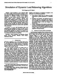
Fig. 2. Cuts Computation
Consider, for instance, Figure 2. The left part of the figure shows the old partition of the domain, which recorded in the cut-array. In the figure, each sub-domain includes a reference to the process owning the sub-domain and the current load of that process. This information, gathered during the trade off evaluation step, is exploited to compute the optimal amount of elements to assign to each process, 25 in the considered example. In the right part of the figure, the new cuts are shown through dashed lines. It is worth noticing that the exact location of the cuts intersecting a sub-domain Dom i , can be determined only by the process Pi owning Domi . Since any other process Pj , j 6= i, does not know the exact location of the elements in Domi , Pj can only determine the number of cuts of the new partition intersecting Domi . During this step, each process Pi builds a list, ListCuts and an array, Receivecuts. Listcuts stores the coordinates of all the cuts intersecting its domain. Receivecuts is an n elements array. Its j-th position records the number of cuts intersecting Domj , for any j 6= i. Consider again Figure 2. Process P1 computes the coordinates of the cuts that intersects the first sub-domain of the old partition and stores them in its Listcuts. All other processes store the value 2 in the first position of their Receivecuts array.
The code implementing this step is shown in Figure 3. We suppose that the variable TotBalance and Optbalance store, respectively, the total number of elements of the grid and the optimal amount of work to be assigned to each process. The i-th position of the array ElPart records the current load of process Pi .
Tot = TotBalance; Diff= OptBalance; i =0; CutPos=0; Listcuts = ∅; while Tot>0 if (Elpart[i]