Load Balancing of Java Applications by Forecasting ... - CiteSeerX

Load Balancing of Java Applications by Forecasting Garbage Collections A. Omar Portillo-Dominguez∗ , Miao Wang∗ , Damien Magoni† , Philip Perry∗ , and John Murphy∗ ∗ Lero,

School of Computer Science and Informatics, University College Dublin, Ireland † LaBRI – CNRS, University of Bordeaux, France e-mail: [email protected], [email protected], [email protected], [email protected], [email protected]

Abstract—Modern computer applications, especially at enterprise-level, are commonly deployed with a big number of clustered instances to achieve a higher system performance, in which case single machine based solutions are less cost-effective. However, how to effectively manage these clustered applications has become a new challenge. A common approach is to deploy a front-end load balancer to optimise the workload distribution between each clustered application. Since then, many research efforts have been carried out to study effective load balancing algorithms which can control the workload based on various resource usages such as CPU and memory. The aim of this paper is to propose a new load balancing approach to improve the overall distributed system performance by avoiding potential performance impacts caused by Major Java Garbage Collection. The experimental results have shown that the proposed load balancing algorithm can achieve a significant higher throughput and lower response time compared to the round-robin approach. In addition, the proposed solution only has a small overhead introduced to the distributed system, where unused resources are available to enable other load balancing algorithms together to achieve a better system performance.

I. I NTRODUCTION AND R ELATED W ORK Enterprise applications commonly require to achieve fast response time and high throughput to constantly meet their service level agreements. These applications make wide use of variants of distributed architectures, usually using some form of load balancing to optimise their performance. Since then researchers have made efforts to improve the business intelligence of load balancers to effectively manage workloads. For example, the authors of [11] proposed a technique to estimate the global workload of a load balancer to use this information in the balancing of new workload. Meanwhile, the work on [5] presented a framework for processor load balancing during the execution of application programs. Regarding Java technologies, the authors of [2] enhanced a load balancing algorithm for Java applications by considering the utilisation of the JVM threads, heap and CPU to decide how to distribute the load. Similarly the work in [6] proposes a function to calculate the utilisation of an Enterprise JavaBean (EJB) and then uses this information to balance the load among the available EJB instances. However, Garbage Collection (GC) metrics have not been considered so far. This gap offers an interesting niche which is yet to be exploited. GC is a core feature of Java which automates most of the tasks related to memory management. However, when the

GC is triggered, it has an impact on the system performance by pausing the involved programs. Even though milliseconds pauses caused by GC does not necessarily lead to a harmful problem, delays of hundreds of milliseconds, let alone full seconds, can cause trouble for applications requiring fast response time or high throughput. This is more likely to occur in the Major Garbage Collection (MaGC), which has the most expensive type of GC pauses [15]. Many research studies have provided evidence to quantify the performance costs of the GC. For example, in [18] authors identified the GC as a major factor degrading the behaviour of a Java Application Server (a traditional Java business niche) due to the sensitivity of the GC to the workload. In these experiments the GC took up to 50% of the execution time of the Java Virtual Machine (JVM), involving pauses as high as 300 seconds. The MaGC represented 95% of those pauses on the heaviest workload. Similarly, a survey conducted among Java practitioners [14] reported GC as a typical area of performance issues in the industry. For these reasons, it is commonly agreed that the GC plays a key role in the performance of Java systems. The goal of this work is to predict the MaGC events and use this information in the decision making process of a load balancer to improve the system performance. Our solution consists of two algorithms. A load balance algorithm which avoids sending any incoming workloads to the application nodes which are likely to suffer MaGC, and an forecast algorithm to predict the MaGCs. The experiment results have shown that this strategy offers a significant performance gain: The average response time of the tested applications decreased between 74% and 99%, while the average throughput increased between 4% and 51%. In summary, the contributions of this paper are: 1) A novel load balance algorithm that uses MaGC forecasts to improve the performance of distributed Java systems. 2) A novel forecast algorithm that enables Java systems to predict when a MaGC event will occur. 3) A validation of the algorithms consisting of a prototype and two experiments. The first proves the accuracy of the MaGC forecast. The second demonstrates the performance benefits of using the forecast for load balancing.

II. BACKGROUND Memory Management in Java. GC is a form of automatic memory management which offers significant software engineering benefits over explicit memory management: It frees programmers from the burden of manual memory management, preventing the most common sources of memory leaks and overwrites [17], as well as improving the programmer’s productivity [9]. Despite these advantages, the GC comes with a cost (as discussed in Section I). Nowadays the most common heap type in Java is the generational heap1 , where the objects are segregated by age into memory regions called generations. New objects are created in the Youngest generation. The survival rates of younger generations are usually lower than those of older ones, meaning that younger generations are more likely to be garbage and can be collected more frequently than older ones. The GC in the younger generations is known as Minor GC (MiGC). It is usually inexpensive and rarely causes a performance concern. MiGC is also responsible of moving the live objects which have become old enough to the older generations, meaning that the MiGC plays a key role in the memory allocation of older generations. The GC in the older generations is known as MaGC and is commonly accepted as the most expensive GC due to its performance impact[15]. Also, it is not possible to programmatically force the execution of the GC[7]. The closest action a developer can perform is to call the method System.gc() to suggest the JVM to execute a MaGC. However, the JVM is not forced to fulfill this request and may choose to ignore it. The usage of this method is discouraged by the JVM vendors2 because the JVM usually does a much better job on deciding when to do GC. Garbage Collection Optimisation & Memory Forecast. Multiple research works have proposed new GC algorithms [3], [4], [10], [12] that have smaller performance impacts on the applications. Even though all these works have helped to reduce the impact of the MaGC, GC remains a concern due to the different factors that can affect its performance. Memory forecast is also an active research topic, looking for ways to invoke a GC only when it is worthwhile. For example, the work presented in [16] exploits the observation that dead objects tend to cluster together to estimate how much space would be reclaimable to avoid low-yield GCs. However memory forecasts alone do not provide enough information to know when the next MaGC would occur.

its workload schedule to avoid the impact of the MaGCs or encourage a MaGC when a resource load (i.e. CPU) is low.

CLIENTS

LOAD BALANCER

INTERNET LOAD BALANCING STRATEGY

SERVERS

MaGC FORECAST

Fig. 1. Adaptive Load Balancer

Among the potential use cases, our work centered on enhancing the performance of a load balancer. This use case was selected because variants of this distributed architecture are commonly used at enterprise-level. This scenario is shown in Figure 1, where the load balancer selects those nodes which are less likely to suffer a MaGC pause as optimal nodes for given workloads. This strategy can keep the system performance safe from any major MaGC pauses. B. Major GC Forecast Algorithm The next sections describe our proposed forecast algorithm. The below definitions will be used on the algorithm discussion: Time is always expressed as the number of milliseconds that have passed since the application started. Young/Old Generation Samples are composed of a timestamp and the usage of the corresponding memory generation. MiGC sample is composed of the start time, the end time and the memory usage before and after the latest MiGC event. Observations are used in a statistical context and are composed of one independent and one dependent values. When the dependent value does not contain historical data, the observation is referred as a forecast observation. Steady state is the state an application reaches after the JVM finishes loading all its classes. It is assumed that this state has been reached if the number of loaded classes remain unchanged for a certain number of consecutive samples.

III. P ROPOSED S OLUTION A. Use case: Adaptive Load Balancer In a distributed Java system, it is preferable that the occurrence of MaGCs in the individual nodes do not affect the performance of the system. To achieve this goal, a system can take different actions. For instance, a system might change 1 http://www.oracle.com/technetwork/java/javase/memorymanagement-

whitepaper-150215.pdf 2 http://docs.oracle.com/cd/E13150 01/jrockit jvm/jrockit/geninfo/devapps/codeprac.html

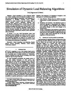
Fig. 2. MaGC Forecast Process - Overview

1) Algorithm Overview: Figure 2 depicts an overview of the algorithm, which is composed of five main phases. First the Initialisation which sets the parameters required by the

algorithm. After it occurs, the other phases are iteratively done to produce MaGC forecasts continuously: New samples are retrieved from the monitored JVM in the Data Gathering phase. Then new observations are generated using the new samples in the Observations Assembly phase. Next the Forecast Calculation occurs. Finally, the logic awaits a Sampling Interval before a new iteration starts. This loop continues until the monitored application finishes. Our algorithm is designed to work on generational heaps, as it is the most common type of Java heap. It only uses standard data that can be obtained from any JVM (such as GC) to make it easy to implement either within or outside the JVM. If the algorithm is implemented within the JVM, the interaction with potential consumers would be simplified. If it is implemented outside the JVM, the implementation would work with any JVM currently available, facilitating the adoption. 2) Detailed Algorithm: It is presented in Algorithm 1, and its phases are explained in the following sections. Algorithm 1: MaGC Forecast Input: Sampling Interval, Forecast Window Size, Warm-up Window Size Output: Forecast time of the next MaGC event 1 steadyState := not reached 2 while forecast is needed do 3 Get new OldGen sample 4 if steadyState is not reached then 5 Get new loaded classes sample 6 if warm-up period is over then 7 steadyState := reached

14

Get new MiGC sample Calculate new memory deltas Update memory totals Generate new observations if steadyState is reached then Forecast memory pending to be allocated Forecast time of the next MaGC event

15

Wait the Sampling Interval

8 9 10 11 12 13

Initialisation. Here the configuration parameters are set: • Sampling Interval: How often the samples are collected. • Forecast Windows Size (FWS): How many observations are used as historical data in the forecast calculation. • Warm-up Window Size: How many samples are used to determine if the application has reached its steady state. Data Gathering. Its objective is to capture an updated snapshot of the monitored JVM. It starts by collecting a new Old Generation sample. Then, if the application has not reached the steady state yet, a new loaded classes sample is collected and its history is reviewed. If the warm-up period is over, a flag is set to indicate this. Later a new MiGC sample is collected and added to the MiGC history. After having samples from at least two MiGCs, the next metrics are calculated: • Time between MiGCs (∆ TM iGC ): How much time elapsed between the latest two MiGCs.

YoungGen Memory Allocation (∆ YMAM iGC ): How much memory was used to create new objects between the latest two MiGCs. • OldGen Memory Allocation (∆ OMAM iGC ): How much OldGen Allocation occurred because of the latest MiGC (meaning that some objects have became old enough to be moved to the OldGen by the latest MiGC). The above metrics are added up into their respective totals (e.g., Total Time between MiGCs) to keep track of how the metrics grow through time. This data is the key input of the regression models used by the algorithm, as explained below. Observations Assembly. Two types of observations are generated and added to their histories. Each is composed of one independent (y axis) and one dependent (x axis) values: The first type (YoungGen-OldGen) captures the relationship between the memory allocation rates (MAR) in the Young and Old Generations. This captures how the Old Generation grows (eventually leading to a MaGC) in relation to the object allocations requested by the application (which occur in the Young Generation). In this observation the dependent value is the Total YoungGen Memory Allocation and the independent value is the Total OldGen Memory Allocation. The second type of observation (Time-YoungGen) captures the relationship between the time and the Young MAR. Here the dependent value is the Total Time between MiGCs and the independent value is the Total YoungGen Memory Allocation. •

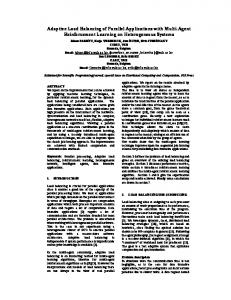
Fig. 3. Old memory exhaustion forecast

Forecast Calculation. This phase first evaluates if the application has reached the steady state. If so, two projections are calculated using linear regression models (LRM). The first projection corresponds to how much memory allocation needs to occur in the Young Generation before the free memory in the Old Generation gets exhausted (hence triggering a MaGC). This is calculated by initializing a LRM with a subset of YoungGen-OldGen observations (defined by the FWS) and then feeding the LRM with a forecast observation whose independent value is the sum of the current Total OldGen Allocation and the free OldGen memory. This is shown in Figure 3. In this example, the free OldGen memory is 1,000MB. As our Total OldGen Allocation is also 1,000MB, the independent value of our forecast observation is 2,000MB. Using the observations within the FWS (the rounded rectangle), the LRM

predicts how much memory allocation needs to occur in the YoungGen before the next MaGC occurs (4,500MB). The second projection is the core output of this algorithm: The MaGC forecast time. It is calculated by initializing a LRM with a subset of Time-YoungGen observations and feeding it with a forecast observation whose independent value is the result of the first projection. This is represented in Figure 4. Using the observations within our FWS, the LRM predicts when the necessary memory allocation in the YoungGen will occur (4,500MB in our example), consequently triggering the next MaGC (around the millisecond 13,000 in our example).

variable) which counts the number of evaluated nodes to prevent an infinite loop in case all nodes are about to suffer a MaGC within the MaGC Threshold. If this occurs, the algorithm would behave as a normal round robin algorithm. Algorithm 2: MaGC-Aware Load Balancing Input: Number of available nodes avNodes, MaGC Threshold maGCThres Output: Next available node (nextNode) 1 indexN extN ode := 0 2 f orecastT ries := 0 3 while load balance adaptiveness is needed do 4 nextN ode := undefined 5 while nextNode is undefined do 6 indexN extN ode := indexNextNode+1 7 if indexN extN ode >avNodes then 8 indexN extN ode := 1 9 10 11

12

13 14 15

Fig. 4. MaGC event forecast

Sampling Wait Period. Finally, the process waits the number of milliseconds configured in the Sampling Interval before starting the next round of iterative steps of the algorithm. C. MaGC-Aware Load Balancing To assess the performance benefits that can be achieved by adapting the load balancing based on the MaGC forecast information, we modified the well-known round robin load balancing algorithm3 . Our proposed algorithm is presented in Algorithm 2. It requires two inputs: The Number of available nodes from which the algorithm will select the next node to send workload; and the MaGC Threshold, which is the time threshold when a node stops being considered a feasible candidate because the next MaGC is too close. For example, if the MaGC Threshold is 5 seconds and the current time is 4:00:00PM, any nodes which report a MaGC forecast between 4:00:00PM and 4:00:05PM will be skipped as their forecasts fall within the configured MaGC Threshold. When compared against the normal round robin, our algorithm has two differences. The main one is that it performs an additional check to adapt the selection of the next node to a close MaGC event. This check reviews if the pre-selected node (as per the normal round-robin logic) will suffer a MaGC within the MaGC Threshold. If it does, the node is skipped and the next available node is evaluated (lines 11 to 15). The second change is an escape condition (the forecastTries 3 http://publib.boulder.ibm.com/infocenter/wsdatap/4mt/

topic/com.ibm.dp.xa.doc/administratorsguide.xa35263.htm

16 17 18 19 20

nextN ode := indexNextNode if f orecastT ries