address this challenge, we present LOADED, a one-pass al- gorithm for ..... Update frequency and correlation coefficients for ) in the hash table. If 2936587( @ ...
LOADED: Link-based Outlier and Anomaly Detection in Evolving Data Sets Amol Ghoting, Matthew Eric Otey and Srinivasan Parthasarathy The Ohio State University ghoting, otey, srini @cis.ohio-state.edu �
�
Abstract Detecting outliers or anomalies efficiently is an important problem in many areas of science, medicine and information technology. Applications range from data cleaning to fraud and intrusion detection. Most approaches to date have focused on detecting outliers in a continuous attribute space. However, almost all real-world data sets contain a mixture of continuous and categorical attributes, and the categorical attributes are either ignored or handled in an ad-hoc manner by current approaches, resulting in a loss of information. The challenge is to efficiently identify outliers in mixed attribute data sets under a variety of constraints, such as minimizing the time to respond, and adapting to the data influx rate. To address this challenge, we present LOADED, a one-pass algorithm for outlier detection in evolving data sets containing both continuous and categorical attributes. LOADED is a tunable algorithm, wherein one can trade off computation for accuracy so that domain-specific (e.g. intrusion detection) response times are achieved. Experimental results validate the effectiveness of our schemes over several real data sets. LOADED provides very good detection and false positive rates, which are several times better than those provided by existing distance-based schemes.
1 Introduction Webster’s Dictionary defines an outlier as “one which lies, or is, away from the main body.” In the context of this work this can mean that an outlier is a sample point that is distinct from most, if not all, other points in the data set. The problem of efficient outlier detection has recently drawn increased attention due to its wide applicability in areas such as fraud detection [5], intrusion detection [7, 25], data cleaning [23, 8], detecting anomalous defects in materials [14], and clinical diagnosis [22]. There are several approaches to outlier detection. One approach is that of model-based outlier detection, where the data is assumed to follow a parametric (typically univariate) distribution [2]. Such approaches do not work well in even moderately high dimensional spaces and finding the right model is often a difficult task in its own right. To overcome these �
This work is supported in part by an NSF CAREER grant (IIS-0347662) and an NSF ACR grant (ACI-0234273)
limitations, researchers have turned to various non-parametric approaches including distance-based approaches [3, 15] and density-based approaches [6, 20]. However, there are several challenges that need to be addressed. First, almost all non-parametric approaches rely on some well-defined notion of distance to measure the proximity between two data points. However, many real-world data sets contain not only continuous attributes, but categorical attributes as well, which have serious implications for a welldefined notion of distance. Simply disregarding categorical attributes in such scenarios may result in the loss of information important for effective outlier detection. Second, an outlier detection scheme needs to be sensitive to response time constraints imposed by the domain. For instance, an application such as network intrusion detection requires on-the-fly outlier detection. Most existing distancebased approaches require multiple passes over the data set which, if not impossible, are prohibitive in such a scenario. In this paper, we present work addressing the above challenges. Specifically, we make the following contributions: First, we define a metric that allows for efficient determination of (a) dependencies within a categorical attribute space, (b) dependencies within a continuous attribute space and (c) dependencies between categorical and continuous attributes. Second, we present an outlier detection algorithm named LOADED (Link-based Outlier and Anomaly Detection in Evolving Data sets) that is based on this metric. Third, we evaluate LOADED for detection quality and scalability on several real data sets. The remainder of this paper is organized as follows. We first examine related work in Section 2. In Section 3, we present our outlier detection scheme. We present our experimental results in Section 4. Finally, we conclude with directions for future work in Section 5.
2 Related Work An approach for discovering outliers using distance metrics was first presented by Knorr et al. [15, 16, 17]. They define a point to be a distance outlier if at least a user-defined fraction of the points in the data set are further away than some user-defined minimum distance from that point. They primarily focus on data sets containing only real valued attributes in their experiments. Related to distance-based methods are
methods that cluster data and find outliers as part of the process of clustering [13]. Points that do not cluster well are labeled as outliers. This is the approach used by the ADMIT intrusion detection system [25]. A clear limitation of clustering-based approaches to outlier detection is that they require multiple passes to process the data set. Recently, density-based approaches to outlier detection have been proposed [6]. In this approach, a local outlier factor (LOF) is computed for each point. The LOF of a point is based on the ratios of the local density of the area around the point and the local densities of its neighbors. The size of a neighborhood of a point is determined by the area containing a user-supplied minimum number of points (MinPts). A similar technique called LOCI (Local Correlation Integral) is presented in [20]. LOCI addresses the difficulty of choosing values for MinPts in the LOF technique by using statistical values derived from the data itself. Most methods for detecting outliers take time that is at least quadratic in the number of points in the data set, which may be unacceptable if the data set is very large or dynamic. Bay et al. [3] present a method for discovering outliers in near linear time. In the worst case, the algorithm still takes quadratic time, but the author reports that the algorithm runs very close to linear time in practice. A comparison of various anomaly detection schemes is presented in [18]. Its focus is on how well different schemes perform with respect to detecting network intrusions. The authors used the 1998 DARPA network connection data set to perform their evaluation, which is the basis of the KDDCup 1999 data set used in our experiments [11]. They found detection rates ranging from a low of 52.63% for a Mahalanobis distance-based approach, to a high of 84.2% for an approach using support vector machines.
3 Algorithms Key Challenges: Our work is motivated by the following questions: First, how does one model categorical attributes in the outlier detection process? Put another way, what is a good distance metric in this space? One approach could be to arbitrarily assign numeric values for each nominal categorical value, and ordinal categorical attributes can be assigned numbers according to their ordinality. However, these values may be meaningless when treated as continuous values by a distance-based scheme, and the problem escalates if there are many such categorical attributes. This can lead to poor detection and high false positive rates [18]. To address this problem, we develop a link-based approach to model similarity between data points. The second question is how does one find the overall distances and correlations in the combined categorical and continuous attribute space? Such correlations may be extremely important to model anomalous activity. One approach could be to find distances in the two data spaces (continuous and categorical) separately and then combine them in some man-
ABC abd
UPPERCASE BOLD itemsets are frequent. lowercase italic itemsets are infrequent.
AB AC BC AD bd
Points: P1: (A, B, C); Score = 0 P2: (A, B, D); Score = 1 3
1 2
�
5 6
Itemsets touched by LOADED for P1 Itemsets touched by LOADED for P2
A B C D
Figure 1. Lattice management in LOADED
ner as has been proposed by others [12]. However, such an approach is not entirely appropriate as it is unlikely to capture the dependencies across the two spaces, which may be essential. We address this issue by maintaining correlation matrices for the continuous attributes for different combinations of categorical attributes. Links in a categorical attribute space: Informally, two data points ��� and ��� are considered linked if they are considerably similar to each other. Moreover, associated with each link is a link strength, which captures the degree of linkage, and is determined using a similarity metric defined on the two points. This is a domain independent definition of a link. We consider a data set � in which, each data point (record) � � has � categorical attributes. We represent � � as an ordered set �
����������������������� �� � ����!"�$#$#�#%�� & ����������'�����)(*�+�� �� � �)(,!�- consisting of � attribute-value pairs. Specifically, we define two data points � � and � � to be linked in a categorical attribute space, if they have at least one attribute-value pair in common. The associated link strength is equal to the number of attribute-value pairs shared in common between the two points (Note that this definition is similar to that of the Hamming distance). Using these definitions, we define an outlier in a categorical attribute space as a data point that has either (a) very few links to other points or (b) very weak links to other points. A score function that would generate high scores for outliers would assign scores to a point that are inversely proportional to the sum of the strengths of all its links. To estimate this score efficiently, we rely on ideas from frequent itemset mining. Let . be the set of all possible attribute-value in the data set � . Let /102 4365 387:9*;�=?�4�@
.�!BA Cpairs �ED �%F ��H G � 3 � # ������4����� ���J0K I 3 � # ������������ ����- , the set of all itemsets, where an attribute only occurs once per itemset. We define L � � M3�! as the number of points �"� in the data set where 3ON �"� , otherwise known as the support of 3 . We also define P 3@P as the number of attribute-value pairs in 3 . We can then define our score function as:
=?Q%;��)� � � � !R01S T4UWV$X
Y[Z
P 3"P
5 L � � E3�!]\ L4^
where the user-defined threshold L is the minimum support or, using our link terminology, the minimum number of links. The score is proportional to the number of infrequent itemsets, and inversely proportional to the size of those infrequent itemsets (i.e. the link strength). The score function has the
following characteristics: A point with no links to other points will have the highest possible score. A point that shares only a few links, each with a low link strength, will have a high score. A point that shares only a few links, some with a high link strength, will have a moderately high score. A point that shares several links, but each with a low link strength, will have a moderately high score. Every other point will have a low to moderate score. We note that the function L � �
3�! has the downward-closure property, otherwise known as the Apriori property.
� Lemma 1 If L � � E 3�!
L then L � � E 3��E! � L C 3�� N 3 .
Example: The score estimation Z process is illustrated as follows: Consider two points 9 and 9�� as shown in Figure 1 together with their itemset lattice. Note that Figure 1 only shows the subset Z of the overall itemset Z lattice corresponding and 9�� . For point 9 , all of its subset itemto the points 9 sets are frequent, and thus using function =?Q%;��)��� , its score would be zero (not an outlier). On the other hand, for point 9�� , subset itemsets ��'3 and �%3 are not frequent. Since ��% � 3 � � has size 3 and �'3 has size 2, the resulting score is ��� 0 . Dealing with Mixed Attribute Data: Thus far, we have presented an approach to estimate a score for a point in a categorical data space. As motivated previously, we would like to capture the dependencies between the continuous and categorical attributes in a domain-independent manner. If the expected dependencies between categorical and continuous data are violated by a point, then it is most likely an outlier. We choose a unified approach to capture this dependence. We incrementally maintain a correlation matrix [10] that stores Pearson’s Correlation Coefficient between every pair of continuous attributes. This matrix is maintained for each itemset in / . This is clearly unrealistic in terms of memory requirements for high dimensional data sets and we relax this requirement towards the end of this section. Furthermore, we store a discretized representation of the true correlation coefficient such that each value is stored in a byte. We maintain 256 equi-width bins to represent the range (-1,1). Since we are maintaining this matrix for each itemset, we are inherently capturing the dependence between the values in the categorical and continuous data spaces. A point is defined to be linked to another point in the mixed data space if they are linked together in the categorical data space and if their continuous attributes adhere to the joint distribution as indicated by the correlation matrix. Points that violate these conditions are defined to be outliers. We modify our score function for mixed attribute data as follows.
Procedure: Find Outliers Input: FrequencyThreshold, CorrelationThreshold, Score, ScoreWindowSize, �������������� Output: Outliers discovered in one pass For� each incoming point p: = Enumeration � of all itemsets of size �������������� for point p For each ��� Get frequency count "!$#&% for � from the hash table Update frequency and correlation coefficients for � in the hash table If '!$#&%�( FrequencyThreshold
)+*&, !-# H )+*&, !-#/.12 3-0 2
�
�
Add all subsets of � of size 4 �54-6 into If these subsets of � do not have an entry in the hash table Get precise a frequency count from 7������������� itemsets Insert frequency count into hash table Else If number of continuous attribute pairs that disagree with the correlation coefficients 8 CorrelationThreshold
)9*&, !$# H )+*&, !-#�.:2 3-0 2 � Add all subsets of � of size 4 �;4-6 � into If these subsets of � do not have an entry in the hash table Get precise a frequency count from �������������� itemsets
Insert frequency count into hash table End For + ) & * , !-#�8=< Avg. score in ScoreWindow >� Score ? If Flag as Outlier Else Normal Update the Score window of size ScoreWindowSize if the point is normal End For end
Figure 2. The LOADED Algorithm for outlier detection
=?Q%;��)� � � ? ! 0
S T4UWV$X
Y[Z
P 3"P
5 C1 @ C2 ! A C3 is true^
where C1: L � � M3�!]\ L , C2: at least ACB of the correlation coefficients disagree with the distribution followed by the continuous attributes for point �"� , and C3: C1 or C2 hold true for every superset of 3 in �"� . Condition C1 is the same condition used to find outliers in a categorical data space using =RQ%;��)� � . Condition C2 adds continuous attribute checks to =RQ%;��)� � . Condition C3 is a heuristic and allows for more efficient processing because if an itemset does not satisfy conditions C1 and C2, then none of its Z subsets will be considered. In other words, for point 9 5 ED �GF �$H ! in Figure 1, if the itemset DIF7H is frequent and if correlation coefficients for itemset Z D�F7H agree with the continuous attribute values in point 9 (within a certain threshold), none of its subset itemsets D�F �-F7H �-DIH �GD �GF �-H need to checked. The rationale for C3 is as follows. First, as stated by the Apriori property in Lemma 1, subsets of frequent itemsets will also be frequent and thus, will not satisfy C1. Second, intuitively, correlation coefficients tend to be less discriminatory as the size of the itemset is reduced and thus, are less likely to satisfy C2. The LOADED Algorithm: LOADED finds outliers based on the score estimation function =?Q%;��)� . It also provides extensions to operate over dynamic data and supports intelligent itemset lattice management. Score estimation using LOADED: The LOADED algorithm for outlier detection is presented in Figure 2. The score function =?Q%;��)� requires that we iterate over all possible itemsets in 9*;�=?�4�@ � � ! . One approach to maintaining frequency counts for these subsets would be use the Lossy
Counting approach proposed by Manku and Motwani [19]. Using this approach, we would need to update frequency counts for each possible subset on a per-point basis, which is an expensive operation. Another approach to the problem would involve using a disk-based approach [9]. Using this approach, everything below the negative border in the lattice will need to be maintained in memory and frequency counts for the remaining infrequent itemsets will be retrieved from the disk as and when needed, which too is an expensive operation. One of the ways to make the algorithm efficient is to minimize the number of itemsets in the itemset lattice that we must examine when a new point arrives. Lemma 1 states the Apriori property that if an itemset is frequent then all of its subsets must also be frequent. An anomaly score for a point is calculated based on the number of infrequent itemsets that it contains (as per function =?Q$;���� � ). Furthermore, due to condition C3, we need only access all itemsets at or above the positive border of the itemset lattice. Our algorithm works as follows:
��������� �
frequency counts of their respective supersets. However, itemset BD is not frequent. As before, we increment the frequency count of item BD and examine its subsets, B and D. B and D are both frequent, so we just increment their respective frequency counts and move on to the next point. Note that in our algorithm, we do not have to examine all of the subsets of itemset ABD.
�
4. If the itemset is frequent, we check that the continuous attributes of the point are in agreement with the distribution determined by the correlation matrix using the CorrelationThreshold (Estimating the level of agreement is a well studied problem in statistics [24]). If so, we will not increase the score. Otherwise, we increase the score, again by a value inversely proportional to the size of the itemset. Z Furthermore, we find all subsets of of size and insert these into . P P
� � 5. If
�
�
� �
�
�
�
�
� �
Lemma 2 The frequency count for any itemset 7 can be precisely estimated using frequency counts from all � D itemsets in .
������� � �
��������� �
In this way, in the worst case, our algorithm examines the itemsets between � D and the positive border of the lattice. The following example (Figure 1) illustrates step 3 of our algorithm. Note that in Figure 1, frequent itemsets are labeled using uppercase characters, while infrequent itemsets are labeled using lowercase characters. Consider the points 9 � 0 ED �GF �$H ! and 9 0 D �-F �+/ ! . The three-itemset corresponding to 9 � is frequent, so we only need to increment the frequency count of itemset ABC in the lattice. As for 9 , ABD is not frequent. Therefore, we increment the frequency count of ABD and examine its subsets AB, AD, and BD. AB and AD are frequent, so we only have to increment their respective frequency counts. Note that the frequency counts of these sets can be derived from the
is not empty go to step 2, else continue.
�
, we increment its fre-
3. We check if ’s frequency is less than FrequencyThreshold. If so, we increase the score by a value inversely proportional to the size of the itemset, as is dictated by the score function. Furthermore, we find all subsets of Z of size P P and insert these into . If has recently become infrequent, there is a possibility that some subsets of may not have an entry in the hash table. We use the following lemma to precisely estimate the frequency count for any subset of .
�
6. We maintain all reported scores over a recent window of size ScoreWindowSize and calculate the average score in the window. If the total score for the point is greater than Score average score, then we flag the point as an outlier.
1. For each point, we enumerate all possible itemsets with a size of � D 0 � into a set . 2. For each of the itemsets 7 quency count in the lattice.
�
Extensions for Dynamic Data: As motivated previously, several applications (e.g. network intrusion detection) demand outlier detection over dynamic data. In order to capture concept drift and other dynamics of the data, we need to update our model to capture the most recent trends in the data. We achieve this by introducing a bias towards recent data. We maintain the itemsets together with their frequency counts in a hash table and the bias is introduced in the following two ways. First, we maintain an itemset together with its frequency count in the hash table only if it appears at least once every points. Second, the frequency for every itemset in the hash table will be decremented by a value every points. We apply these biases using smart hash-table management coupled with a down-counting approach described in Figure 3. For every points, we create a new hash table with index � 3�� � and delete the oldest hash table with index (�"3 � � � ). Thus, at every instant in time, we maintain at most two hash tables. We estimate the frequency for an itemset based on the its frequency in the two hash tables. Moreover, for every points, relevant itemsets will have their frequencies biased with a value of . The oldest hash table is deleted every points and the two most recent hash tables will contain all the relevant itemsets with their biased frequencies. Single-Pass vs Multi-Pass LOADED: For an application such as network intrusion detection, providing an interactive response time is crucial. This enforces a one-pass processing requirement over the data set and the score is estimated using itemset frequency counts maintained over a recent window of time. On the other hand, an application may need a
�
�
�
�
��
���
�
���
���
Hash Table Management: Let be the index of the point that just arrived If �������� � , Then create a new hash table with index ������ delete the hash table with index ����������
LOADED’s time complexity grows linearly in the size of the data set and quadratically in the number of continuous attributes. We partially alleviate the complexity associated with the expensive operation of lattice management by operating between � D and the positive border. Moreover, a decade of research [1, 26] has shown that under practical considerations, an itemset lattice can be managed in an efficient and scalable fashion, which is also evident in our experimental results.
��������� �
Frequency Estimation: When estimating the frequency for an itemset from a point with index : If an itemset for the ���� point is found in hash table with index ������ Increment and use the freq. from this hash table Else If itemset is found in hash table with index ���������� insert it into the hash table with index ������� , set freq = freq in table �������������!#"$�%��&(' and then use this freq. Else insert it into the hash table with index ������� with freq. = 1 Figure 3. Algorithm for hash table management and frequency estimation
higher detection accuracy, arguing for a two-pass approach. In the first pass, we find itemset frequency counts over the entire data set and in the second pass, we find outliers based on what we have learned. The two-pass approach is beneficial as points that were mistaken as outliers during the first pass (due to a lack of information about the entire data set) will not be flagged as outliers in the second pass. Approximation Scheme: As it stands, our algorithm maintains and examines the itemset lattice beginning at � D 0 � down to the positive border, and for each itemset in that lattice, there is a correlation matrix whose size is proportional to the the square of the number of continuous attributes. Maintaining this lattice and the corresponding matrices can consume a large amount of memory, even with the optimizations considered in LOADED. Furthermore, the time it takes to check if a point is an outlier is proportional to the number of lattice levels between � and the positive border. For some applications, the amount of memory used by our algorithm or the time taken to determine if a point is an outlier may be too costly. In this case, it would be better to use a faster and more memory-efficient algorithm that approximates the anomaly score. Given two 1-itemsets .>� and . , the frequency for the 2itemset .)�)A]. is bounded by the smaller of the frequencies for .)� and . . As a result, the frequencies of the lower order itemsets serve as good approximations for the frequencies of the higher order itemsets. We consider approximations by maintaining itemsets only up to a certain level � D . An approximate scheme such as this will provide improved execution time as a smaller subset of the lattice needs to be considered. However, the accuracy of the algorithm will decrease. In the general case, accuracy improves as � D increases. We empirically validate this in the next section.
����� ��� �
����� ��� �
��������� �
4 Experimental Results Setup: We ran our experiments on system with a 1GHz Pentium III processor and 1GB RAM running Linux kernel 2.4. We evaluate LOADED 1 using the following real data sets2 : (a) KDDCup 1999: The 1999 KDDCup data set [11] (4,898,430 training and 51425 testing data instances with 32 continuous and 9 categorical attributes) contains records that represent connections to a military computer network where there have been multiple attacks and intrusions by unauthorized users. Each record is also labeled with an attack type. (b) Adult Database: The Adult data set [4] (48,842 data instances with 6 continuous and 8 categorical attributes) was extracted from the US Census Bureau’s Income data set. Each record has features that characterize an individual’s yearly income together with a class label indicating whether the person made more or less than 50,000 dollars per year. (c) Congressional Votes: This data set (435 data instances with 16 categorical attributes) is the 1984 US Congressional Voting Record. Each record corresponds to one Congressional Representative’s votes on 16 issues together with a classification label of Republican or Democrat. Nature of the Discovered Outliers: KDDCup 1999: As described in the previous section, LOADED flags a data point as an outlier using the frequency counts for various combinations of M ������������ �������� �� � �>! pairs in the data set. A fair evaluation of our approach would require outliers to constitute a small fraction (between 1-3%) of the data set. The KDDCup data set however, has a larger fraction of outliers (intrusions). We filter out all the anomalous records from the data set and reinsert them into the data set in a semi-random fashion so that the total number of anomalous records was equal to 2% of the entire data set. The semi-randomness stems from the fact that we maintain the same proportion for different types of intrusions in the original data set and we also insure that attacks that happen in blocks (e.g. DOS attacks) will occur in blocks in the new data set. We compare our approach against ORCA [3] which is a state-of-the-art distance-based outlier detection algorithm with a publicly available implementation. ORCA uses Euclidean distance and Hamming distance as similarity measures for continuous and categori1 For
all experiments unless otherwise noted, we run LOADED with the following parameter settings: FrequencyThreshold=10, CorrelationThreshold=0.3, & Score=10, ScoreWindowSize=40. 2 We have also evaluated LOADED over other real data sets with good results, but due to space limitations those results are not included in this paper.
Attack Type Apache 2 Buffer Overflow Back FTP Write Guess Password Imap IP Sweep Land Load Module Multihop Named Neptune Nmap Perl Phf Pod Port Sweep Root Kit Satan Saint Sendmail Smurf Snmpgetattack Spy Teardrop Udpstorm Warez Client Warez Master Xlock Xsnoop
Detection Rate (10% Training) LOADED/ORCA n/a 94%/63% 100%/5% 28%/88% 100%/21% 100%/13% 42%/3% 100%/66% 100%/100% 94%/57% n/a 92%/1% 94%/8% 100%/100% 0%/25% 45%/12% 100%/13% 33%/70% 75%/9% n/a n/a 24%/1% n/a 100%/100% 50%/1% n/a 48%/3% 0%/15% n/a n/a
Detection Rate (Testing) LOADED/ORCA 100%/0% 90%/100% n/a n/a 100%/0% n/a 28%/0% n/a n/a 100%/75% 100%/40% n/a n/a n/a 20%/100% 100%/18% 100%/3% n/a n/a 100%/1% 50%/50% 21%/0% 52%/0% n/a n/a 0%/0% n/a n/a 50%/66% 100%/100%
Attack Type Apache 2 Buffer Overflow Back FTP Write Guess Password Imap IP Sweep Land Load Module Multihop Named Neptune Nmap Perl Phf Pod Port Sweep Root Kit Satan Saint Sendmail Smurf Snmpgetattack Spy Teardrop Udpstorm Warez Client Warez Master Xlock Xsnoop
Detection Rate (Training) LOADED n/a 91% 97% 33% 100% 100% 37% 100% 100% 94% n/a 98% 91% 100% 0% 53% 100% 33% 72% n/a n/a 22% n/a 100% 49% n/a 43% 0% n/a n/a
Table 1. Detection rates for LOADED (single pass) and
Table 2. Detection rates for LOADED (single pass) on com-
ORCA on 10% KDDCup1999 training data set and complete testing data set
plete KDDCup 1999 training data set
cal attributes respectively. It finds the top- outliers in a data set, with being a user supplied parameter. For an application such as network intrusion detection, ORCA, being a nearest neighbor-based approach, needs the assistance of an oracle to set equal to the number of true outliers in the data set. To this effect, we set equal to the number of outliers in the data set. We are only able to make a comparison between ORCA and LOADED on a 10% subset of the KDDCup 1999 training data set, because ORCA would take time on the order of days to process the entire training data set. Detection rates for the two approaches are reported in Table 1 (Note that “n/a” indicates that the attack was not present in the particular data set). Overall, our detection rates are very good and much higher than those from approaches using a distance-based scheme. This can be attributed to a more effective representation of both categorical data and continuous data in the LOADED approach. The attacks in the training data set for which we do poorly are Phf, Warez Master, FTP Write, IP Sweep, Smurf and Rootkit. For Phf, Warez Master and FTP Write, ORCA is able to provide better detection rates, while for IP Sweep and Smurf, LOADED provides better detection rates, arguing for an ensemble-based outlier detection approach [21]. The remaining intrusions for which we do poorly are detected in a second pass of the algorithm. The rationale for this behavior can be explained by the distribution of their arrivals. For instance, smurf attacks, which tend to be grouped attacks (DOS), arrive in the first part of the data set. In our one-pass
LOADED ORCA
Execution time KDDCup Training Dataset (10%) 469 seconds 212 minutes
Execution time KDDCup Testing Dataset 48 seconds 2 minutes
Table 3. Execution time comparison
algorithm the first few smurf attacks are flagged but the later ones are not since at that point in time only a small part of the data set has been read and the percentage contribution of smurfs is quite high. A similar rationale extends to the other intrusions with low detection rates. On the testing data set our approach is able to detect most of the unknown attacks (a problem for almost all of the KDDCup 1999 participants). For an evaluation of LOADED over the entire KDDCup 1999 training data set, please refer to Table 2 Note that our approach is a general anomaly detection scheme and has not been trained to catch specific intrusions. Once an anomaly is detected, a network administrator can perform a more detailed investigation and develop a signature for this attack, thus facilitating signature-based intrusion detection in conjunction with our approach. All the intrusions reported in the above table are caught in a single pass, since making two passes of the data is infeasible in the domain of network monitoring. Our results are even more impressive when we examine the false positive rate (which we compute as number of normal records flagged as outliers divided by the total number of records in the data set) and execution time. We measure the false positive rate over the original data set with the full set of
35
Execution time (seconds)
Execution time per thousand transactions (ms)
1300 1200 1100 1000 900 800 700 600 KDDCup 1999
500 400 300
30
Adult Database
25 20 15 10 5
1
2
3
4
5
6
7
Number of lattice levels
1
2
3
4
Number of lattice levels
Figure 4. Execution time variation with increase in lattice levels
outliers. Our approach gives us a false positive rate of 0.35%, which is extremely good for anomaly detection schemes, especially considering our high detection rates. ORCA has a false positive rate of 0.43%, but this is not significant considering its lower detection rates. LOADED’ S low false positive rate can be attributed to a better representation for anomalous behavior obtained by capturing the dependence between categorical attributes and their associated continuous attributes. Table 3 compares execution time for LOADED and ORCA. LOADED operates in one-pass with a complexity that grows linearly in the size of the data set, thus facilitating applications like intrusion detection. ORCA, on the other hand, needs multiple passes over the data set and operates with a worstcase complexity that is quadratic in the size of the data set. Furthermore, its execution time is also dependent on the parameter . For the KDDCup testing data set, ORCA takes a relatively small amount of time compared to the KDDCup training data set. This is due to the fact that we select a smaller value of for the testing data set as it has fewer outliers. Adult Database: This data set is processed in two passes. In the first pass, LOADED learns the model and in the second pass, it flags the outliers. We do not process this data set in a single pass since this is a static data set that does not warrant on-the-fly outlier detection. Learning the model in the first pass gives us better global information for the second pass. Here we are unable to make a comparison with ORCA, since this data set does not provide us with labeled outliers. The following data records are marked as the top outliers: (a) A 39 year old self-employed male with a doctorate, working in a Clerical position making less than 50,000 dollars per year (b) A 42 year old self-employed male from Iran, with a bachelors degree, working in an Executive position making less than 50,000 dollars per year (c) A 38 year old Canadian female with an Asian Pacific Islander origin working for the US Federal Government for 57 hrs per week and making more than 50,000 dollars per year Apart from these, the other outliers we find tend to come from persons from foreign countries that are not well represented in this data set. Congressional Votes: As in the previous case, the limited size of the data set warrants a two-pass approach. We are unable
to compare with ORCA because, as in the previous case, this data set does not contain labeled outliers. Many of the top outliers contain large numbers of missing values, though there are examples in which this is not the case. One such example is a Republican congressman, who has four missing values, but also voted significantly differently from his party on four other bills. According to the conditional probability tables supplied with the data set, the likelihood of a Republican voting in a such a manner is very low. Benefits of the Approximation Scheme: To demonstrate the benefits of our approximation scheme, we again consider the KDDCup 1999, Adult and US Congressional Voting Record data sets. In our experiments, we measure the execution time, detection rate and the false positive rate as a function of the number of itemset lattice levels maintained. For execution time, in the case of a one pass approach (for KDDCup), we measure the execution time per 1000 tuples processed, and in the case of two pass approach, we report the overall execution time. For the Adult and Congressional Votes data sets, we define the detection rate as the number of outliers found using only the sub-lattice of itemsets divided by the number of outliers found using the complete lattice. The primary benefit of our approximation scheme is that far better execution times can be achieved if we maintain fewer lattice levels, as can be seen in Figure 4. However, our false positive rates increase and detection rates decrease as the number of lattice levels decrease, as can be seen in Figure 5. From Figure 5, one can see that number of lattice levels has a greater affect on the detection rate in the case of the KDDCup data set than in the other data sets. This can be attributed to larger categorical attribute dependencies being used in the detection process for the KDDCup data set. The other data sets can work reasonably well with smaller lattices. The number of lattice levels maintained does not affect the false positive rate as much as they affect the detection rate. For both the false positive rate and the detection rate, the more information that is used (i.e. the more lattice levels that are maintained), the less likely the system is to make a mistake. We also note that the processing rate per 1000 network transactions is within reasonable response time rates even for a lattice
0.5
False Positive Rate %
1
Detection Rate
0.9 0.8 0.7 0.6 0.5
KDDCUP 1999 Adult Database US Congressional Votes
0.4 0.3
0.45 0.4 0.35 KDDCUP 1999 Adult Database US Congressional Votes
0.3 0.25 0.2
1
2
3
4
Number of lattice levels
1
2
3
4
Number of lattice levels
Figure 5. Detection and false positive rates
level equal to four. Ideally, one would like to tune the application based on the learning curves in an application specific manner, as each application will exhibit a specific dependence behavior. For example, in network intrusion detection, execution time must be minimized to keep pace with the network traffic, and since only one packet of an attack needs to be flagged in order to alert a monitor that an attack is in progress, using fewer lattice levels may be advisable. However, in other domains this might not be the case. Empirically, it appears from Figure 4 that execution time grows near-linearly with the number of lattice levels.
5 Conclusion Applying existing distance-based outlier detection algorithms to mixed attribute data has a major limitation in that distance is ill-defined in the categorical data space. In this paper, we presented LOADED, an algorithm for effective outlier and anomaly detection in such mixed attribute data sets. Our work combines the following key components. First, we define a robust unifying similarity metric that combines a linkbased approach (for categorical attributes) with correlation statistics (for continuous attributes). Data points that violate these dependencies are flagged as outliers. It is a one-pass algorithm that can operate on evolving data sets. Second, since the memory requirements imposed by LOADED can be quite high in large feature spaces, we describe a tunable approximation mechanism that reduces its memory requirements at a small cost to accuracy. Finally, we evaluated LOADED on several real mixed attribute data sets with good results. As part of future work, we are looking to extend the proposed work to reduce the memory requirements of our algorithm even further and to evaluate our work on CISCO Netflow data generated by the OSU Office of Information Technology routers.
6 Acknowledgments We would like to thank Stephen Bay for providing us with his implementation of ORCA.
References [1] R. Agrawal and R. Srikant. Fast algorithms for mining association rules. In VLDB, 1994.
[2] V. Barnett and T. Lewis. Outliers in Statistical Data, 1994. [3] S. Bay and M. Schwabacher. Mining distance-based outliers in near linear time with randomization and a simple pruning rule. In ACM SIGKDD, 2003. [4] C. Blake and C. Merz. UCI machine learning repository, 1998. [5] R. Bolton and D. Hand. Statistical fraud detection: A review. Statistical Science, 2002. [6] M. Breunig et al. LOF: Identifying density-based local outliers. In ACM SIGMOD, 2000. [7] E. Eskin et al. A geometric framework for unsupervised anomaly detection: Detecting intrusions in unlabeled data. In Data Mining for Security Applications, 2002. [8] D. Gamberger, N. Lavraˇc, and C. Groˇselj. Experiments with noise filtering in a medical domain. In ICML, 1999. [9] A. Ghoting and S. Parthasarathy. DASPA: A disk-aware stream processing architecture. In SIAM High Performance Data Mining Workshop, 2003. [10] J. Han and M. Kamber. Data Mining: Concepts and Techniques. Morgan Kaufmann, 2001. [11] S. Hettich and S. Bay. KDDCup 1999 data set, UCI KDD archive, 1999. [12] Z. Huang. Clustering large data sets with mixed numeric and categorical values. In PAKDD, 1997. [13] A. Jain and R. Dubes. Algorithms for Clustering Data. Prentice Hall, 1988. [14] M. Jiang et al. Feature mining paradigms for scientific data. In SIAM Data Mining, 2003. [15] E. Knorr et al. Distance-based outliers: Algorithms and applications. VLDB Journal, 2000. [16] E. Knorr and R. Ng. A unified notion of outliers: Properties and computation. In ACM SIGKDD, 1997. [17] E. Knorr and R. Ng. Finding intentional knowledge of distance-based outliers. In VLDB, 1999. [18] A. Lazarevic et al. A comparative study of outlier detection schemes for network intrusion detection. In SIAM Data Mining, 2003. [19] G. Manku and R. Motwani. Approximate frequency counts over data streams. In VLDB, 2002. [20] S. Papadimitriou et al. LOCI: Fast outlier detection using the local correlation integral. In ICDE, 2003. [21] Byung-Hoon Park and Hillol Kargupta. Distributed data mining: Algorithms, systems, and applications. In Nong Ye, editor, Data Mining Handbook, 2002. [22] K. Penny et al. A comparison of multivariate outlier detection methods for clinical laboratory safety data. The Statistician, Journal of the Royal Statistical Society, 2001. [23] Rulequest Research. www.rulequest.com. [24] J. Rice. Mathematical Statistics and Data Analysis, 1995. [25] K. Sequeira and M. Zaki. ADMIT: Anomaly-based data mining for intrusions. In ACM SIGKDD, 2002. [26] A. Veloso et al. Mining frequent itemsets in evolving databases. In SIAM Data Mining, 2002.