A local mesh refinement technique based on the variational nodal transport method has been developed to account explicitly for strong localised ...
LOCAL MESH REFINEMENT IN REACTOR CALCULATION USING VARIATIONAL NODAL METHOD J.M. Ruggieri*, R. Boyer**, F. Malvagi***, J.Y. Doriath* * C.E.A., CE/Cadarache, DRN/DER/SPRC (FRANCE) *} University of Provence, Mathematics Research Division, Marseille (FRANCE) {***} University of California, San Diego, Climate Research Division (USA)
ABSTRACT A local mesh refinement technique based on the variational nodal transport method has been developed to account explicitly for strong localised heterogeneities in full core calculations. This technique relies on using the partial ingoing surface currents produced during coarse mesh iterations as boundary conditions for fine mesh calculations embedded within the coarse mesh calculations. The outgoing fine mesh partial currents are averaged to serve in the coarse mesh iterations. This method has been developed for 2D XY-geometry and has been tested for a detailed rodded PWR model.
I. Introduction Current 30 core calculation techniques consist of separating the neutronic behaviour in several successive processing steps; at first, very detailed (in energy and space) transport calculations are performed for small regions (usually one or a few assemblies); results are condensed in energy and space to yield coarse mesh few group cross sections. These cross-sections are then used in coarse mesh nil core calculations (usually based on a nodal formulation) which produce coarse mesh fluxes- and reaction rates. Finally, local (usually pinwise) fluxes and reaction rates are reconstructed through some interpolation scheme of the coarse mesh results. Every step in these procedures involves approximations with a limited domain of validity. Of particular concern is the treatment of strong localised heterogeneities such as control rods which in the classical approach are homogenised with the surrounding fuel and moderator regions; the homogenisation treatment usually introduces non negligible errors in the neutronic calculations [1] which might not be acceptable in view of the need to reduce design margins in future reactor concepts. Ideally, strong heterogeneities would be explicitly represented in a complete 3D pin by pin transport calculation of the core; nevertheless this approach would not be practical (or even feasible) on the current generation of computers. The purpose of this paper is to describe and test an approach which should provide the local accuracy of a full core pin by pin calculation, while requiring computing resources almost equivalent to those of a typical nodal calculation; it relies on full core nodal transport calculations along with a localised mesh refinement which allows for an explicit treatment of heterogeneities in the region of interest to the core analyst. The variational nodal method (VNM) developed by E.E. Lewis [1] is used for the nodal transport calculation; the spatial meshing in one or several nodes is refined to represent localized heterogeneities; during the inner iterations, surface ingoing currents from the coarse mesh calculation are projected onto the fine mesh boundaries; an additional iteration loop (using the VNM formalism) is then performed within the fine mesh region and the converged outgoing currents are collapsed on the outer surface to serve in the coarse mesh inner iterations.
617
II. Response Matrices Formulation II. 1 Variational Formulation The response matrices used in VNM [3,4] are derived from the functional for the wilhin-group even-parity transport equation. The functional may be written as a sum over the nodal contributions
V
where y and x are the even- and odd-parity components of ¥ , the angular flux. For each node, the functional is divided into volume and surface contributions
1
V
where f is the scalar flux, and the remaining notation is conventional. I so tropic scattering and group sources are assumed. It may be shown that requiring the functional to be stationary with respect to variations in y and X results the Euler-Lagrange equations that are the even-parity transport equation - Q . V—Q. V\|/(r,Q) + OT|/(r,Q) =
o$(r)+S(r)
within the node and the associated continuity conditions on y and
X(r,Q) =
1
i
across the nodal interfaces.
H.2 Ritz Procedure Formally, the response matrices result from the following Ritz procedure. The even- and odd-parity angular flux contributions are approximated as
and
reTy. In these equations, the ^ and x^y are arrays of unknowns. The spatial basis/and h are complete polynomials and the angular basis g and k are spherical harmonics. To obtain the response matrices, we rewrite the reduced functional in partitioned matrix form
618
where the partitioning of A, s and M is consistent with that of \ and %. Requiring the functional to be stationary with respect to the variations in % then yields
Y
or, solving for the even-parity flux coefficients,
(2) Substituting in the reduced nodal functional Eq. (1) and taking the variation with respect to %, across an interface leads to the requirement that the following quantity be continuous across each interface: VT = M &
(3)
Combining Eq.(2 ) and (3), we have
xVy=M'rA-ls-^M-A-]MrXr. r
(4)
To obtain a response matrix conventional form, we introduced a change of variables
j;=±M-y%±±Xy,
(5)
where 7* are the outgoing and incoming partial current-like moments. Combining Eq. (4) and (5), we may then write the nodal response matrix in the form (6) where
J? = [G+/]-'[G-/]
are also in partitioned form with
G^^M'^M,
and Cy = ±M-A-\
Once the partial current moments are determined, the even-parity flux moments in the node can be determined by
t> = A-ls-2C'(r-J-),
(8)
where the first subvector § of \ contains the scalar flux moments.
619
III. Local mesh Refinement Method III. 1 Solution Algorithm The solution algorithm derives from the Schwartz algorithm [5,6] for domain decomposition problem. For the local mesh refinement method, two meshing levels are used. The first one is the coarse mesh for the global geometry of the reactor (one mesh per assembly) and the second one is the local fine mesh which describes the heterogeneous zone of interest. Once the domain is meshed, the response matrices for each coarse and fine node are calculated. Then iterations are performed. These iterations consist in two loops, the loop over the coarse mesh nodes and the loop over the fine mesh nodes embedded within the coarse mesh calculations. In a given iteration, the first step consists to calculated all the outgoing cunents of the coarse mesh nodes using Eq. (6) excepted for the refined one. This produces the incoming currents at the interfaces between the coarse and the fine mesh. This coarse current is projected onto the fine mesh domain boundary interfaces and it produces the incoming fine current at the boundary. Then the second step of the iteration is performed; the outgoing currents for the fine nodes are calculated with the relationship (6) and the previous boundary incoming fine cunents. This produces the fine outgoing currents at the interfaces between fine and coarse mesh. These currents are used to reconstruct the coarse outgoing currents to update the following iteration on the coarse nvrsh nodes. This algorithm relies on two major approximations which are the basis for the projection and the reconstruction techniques. The following example (see Fig. 1) illustrates the two techniques.
III.2 Partial Currents at the Fine/Coarse Mesh Interfaces Fie. 1: Current Projection on the Interface Between Fine and Coarse Mesh
in" V
r2 J2+
I7 Jl."
v,,
V,4
r,
r
vz
In this example, the outgoing coarse current Jj the node V2 is divided into two incoming fine currents Jf, and/,^. Once the transport calculation over the coarse nodes is done, the coarse current 72+ has the following polynomial form N
Q),
(9)
and this current has to be projected on each interface of the fine mesh Tj and F 2 For this, the fine currents 7,", and 7,~2 are defined, as r.O),
I'=1,2.
k=O
620
(10)
Then, the following functional is considered
(ii) The fine currents components are derived by minimisation of L with respect to each component. This technique produces the following relationships:
(12) *"=o ' r ,
In a similar way, the coarse current components are obtained from the known components of the fine currents and are used to update the iteration on the coarse mesh nodes:
Ju =
!/'
k
~
l
(13)
-'
IV. Numerical Results IV. 1 Geometry Description To test this method, several numerical tests have been performed. The Benchmark presented here is based on cross-sections and geometry data given in the Benchmark Calculations of Power Distribution Within Assemblies [7J. Table 1: The 2-group cross-sections Cell Type u:UO2 x: Guide tube c: Moveabie fission chamber a: Absorber
Dl 1.2 1.2 1.2 1.2
SA1 0.010 0.001 0.001 0.040
SR 0.020 0.050 0.025 0.010
NSF1 0.0050 0 l.E-7 0
D2 0.4 0.4 0.4 0.4
SA2 0.10 0.02 0.02 0.80
NSF2 0.125 0 3.E-6 0
where Dl and D2 are the diffusion coefficients, SA1 and SA2 are the absorption cross-sections, SR is the down-scattering cross-section and NSF1 and NSF2 are the fission cross-sections. In this test case, nine assemblies are considered (see Fig. 2), eight of them being completely homogeneous (UO2 fuel) whereas the central assembly is heterogeneous (see Fig. 3). The problem is treated with reflective boundary conditions (i.e. J=0). Fie. 2: Coarse Mesh XY-Geometrv
UO2
UO2
UO2
UO2
ASSEMBLY
UO2
UO2
UO2
UO2
621
R- • i:
u u u u u u u u u u u u u u u u u
u u u u u u u u u u u u u u u u u
u u u u u a u u a u u a u u u u u
u u u a u u u u u u u u u a u u u
u u u u u u u u u u u u u u u u u
Heterogeneous Assembly
u u a u u a u u a u U
a
u u a u u
u u u u u u u u u u u u u u u u u
u u u u u u u u u a u u 11 u u u u u u u u a u u u u u u u u u u u c u u u u u u u u u u u a u u u u u u u u u u u a u u u u u u u u u u
u u a u u a u u a u u a u u a u u
u u u u u u u u u u u
u u u u u u
u u u a
u u u u u u u u u a u u u
u u u u u a u u a u u a u u u u u
u u u u u u u u u u u u u u u u u
u u u u u u u u u u u u u u u u u
IV.2 Results For the local refinement method, a 3x3 coarse mesh is used for the reactor and the heterogeneous node is described with a local 17x17 mesh refinement. For the reference calculation, a fine mesh calculation (with a 51x51 mesh) using the varialional nodal transport method is used. The calculated keff and the CPU time are presented in Table 2. The errors on the keff are acceptably low and the transport calculation is performed with very reasonable computing time. Table 2: keff and CPU Time
DIFFUSION TRANSPORT
METHOD reference local refinement reference local refinement
k*ff
CPU Time
0.97312 0.97275 0.97503 0.97474
18,2S 1,3s 116s
Ms
Fig. 4 represents the median thermal flux profile of the heterogeneous node and Fig. 5 shows the difference (in %) between the reference flux and the local refined mesh flux for the same profile. These two figures show a very good precision (~ 1%) for the flux distribution in the center of the refined node and also show that the difference between the reference flux and the local refined mesh flux is more important (~ 4%) close to the boundaries between the fine mesh and the coarse mesh. Nevertheless the refined calculated flux is acceptably close to the reference flux. This effect can be due to the errors introduced by the approximations made for the projection and the reconstruction of the incoming and outgoing currents onto the interfaces between fine and coarse mesh. Some other techniques, to define the boundary conditions for the refined node calculations, need to be improved to estimate the real contributions of these approximations for the errors that appear in the local mesh refinement calculation. Finally. Fig. 6 represents the local refined mesh calculated flux distribution within the heterogeneous assembly for the thermal group.
622
Fig. 4: Transport Thermal Flux
Fig. 5: 1- (Refinement Method Flux / Reference Flux) For the Thermal Group
««
5
--
4.5
--
t
--
3.5
--
3
--
2.5
--
a
-
1.5
--
0.5
--
0 -—
Fig. 6: Transport Flux Distribution in the Assembly For The Thermal Group
623
V. Conclusion The local mesh refinement method appears to have good convergence properties which make it applicable to a wide variety of transport core calculations. Its good accuracy in terms of flux distribution within the strong heterogeneous zones in PWR calculations suggests that it can be used to calculate most of the heterogeneities of a reactor (control rod, U02-M0X assemblies, core-reflector boundary, control rod cusping,...) with reasonable computing time. The contributions of the different approximations made in this method have to be defined by testing this method on a large set of heterogeneities.
Acknowledgement The authors wish to thanks P.J. Fink for valuable discussions and comments and G. Palmiotti for the method investigations which form the starting point of this work.
References 1. K.S. Smith, "Assembly Homogenisation Techniques for Light Water Reactor Analysis", Prog. Nucl. Energy, 17,3, 305(1986). 2. I. Dilber and E.E. Lewis, Nucl. Sci. Eng., 91, 132(1985). 3. E.E. Lewis, Nucl. Sci. Eng., 102, 140 (1988). 4. C.B. Carrico and E.E. Lewis, Nucl. Sci. Eng., I l l , 168 (1992). 5. H.A. Schwartz, Gesammelt mathematishe abhandlungen, Springer, Berlin (1980). 6. PL. Lions, "On the Schwartz alternating method I", First Int. Symposium on Domain Decomposition Methods for Partial Differential Equations, SIAM, Philadelphia, USA. 7. C. Cavarec, J.C. Lefebvre, J.F. Perron, D. Verwaerde and J.P. West, "Benchmark Calculations of Power Distribution within Assemblies", Int. Meeting 1993, Karlsruhe, Germany.
624