Joint 45th International Symposium on Robotics (ISR) and 8th German Conference on Robotics (ROBOTIK), Munich, June 2014.
Local Navigation in Rough Terrain using Omnidirectional Height Max Schwarz,
[email protected] Sven Behnke,
[email protected] Rheinische Friedrich-Wilhelms-Universit¨at Bonn Computer Science Institute VI, Autonomous Intelligent Systems Friedrich-Ebert-Allee 144, 53113 Bonn
Abstract Terrain perception is essential for navigation planning in rough terrain. In this paper, we propose to generate robotcentered 2D drivability maps from eight RGB-D sensors measuring the 3D geometry of the terrain 360◦ around the robot. From a 2.5D egocentric height map, we assess drivability based on local height differences on multiple scales. The maps are then used for local navigation planning and precise trajectory rollouts. We evaluated our approach during the DLR SpaceBot Cup competition, where our robot successfully navigated through a challenging arena, and in systematic lab experiments.
1
Introduction
Most mobile robots operate on flat surfaces, where obstacles can be perceived with horizontal laser-range finders. As soon as robots are required to operate in rough terrain, locomotion and navigation becomes rather difficult. In addition to absolute obstacles, which the robot must avoid at all costs, the ground is uneven and contains obstacles with gradual cost, which may be hard or risky to overcome, but can be traversed if necessary. To find traversable and cost-efficient paths, the perception of the terrain between the robot and its navigation goal is essential. As the direct path might be blocked, an omnidirectional terrain perception is desirable. To this end, we equipped our robot, shown in Fig. 1, with eight RGB-D cameras for measuring 3D geometry and color in all directions around the robot simultaneously. The high data rate of the cameras constitutes a computational challenge, though. In this paper, we propose efficient methods for assessing drivability based on the measured 3D terrain geometry. We aggregate omnidirectional depth measurements to robot-centric 2.5D omnidirectional height maps and compute navigation costs based on height differences on multiple scales. The resulting 2D local drivability map is used to plan cost-optimal paths to waypoints, which are provided by an allocentric terrain mapping and path planning method that relies on the measurements of the 3D laser scanner of our robot [10]. We evaluated the proposed local navigation approach in the DLR SpaceBot Cup—a robot competition hosted by the German Aerospace Center (DLR). We also conducted systematic experiments in our lab, in order to illustrate the properties of our approach.
Figure 1: Explorer robot for mobile manipulation in rough terrain. The sensor head consists of a 3D laser scanner, eight RGB-D cameras, and three HD cameras.
2
Related Work
Judging traversability of terrain and avoiding obstacles with robots—especially planetary rovers—has been investigated before. Chhaniyara et al. [1] provide a detailed survey of different sensor types and soil characterization methods. Most commonly employed are LIDAR sensors, e.g. [2, 3], which combine wide depth range with high angular resolution. Chhaniyara et al. investigate LIDAR systems and conclude that they offer higher measurement density than stereo vision, but do not allow terrain classification based on color. Our RGB-D terrain sensor provides high-resolution combined depth and color measurements at high rates in all directions around the robot. Further LIDAR-based approaches include Kelly et al. [6], who use a combination of LIDARs on the ground vehicle and an airborne LIDAR on a companion aerial vehicle. The acquired 3D point cloud data is aggregated into a 2.5D height map for navigation, and obstacle cell costs are computed proportional to the estimated local slope, similar to our approach. The additional viewpoint from the arial vehicle was found to be a great advan-
tage, especially in detecting negative obstacles (holes in the ground), which cannot be distinguished from steep slopes from afar. This allows the vehicle to plan through areas it would otherwise avoid because of missing measurements, but comes at the price of an increased system complexity. Structured light has also been proposed as a terrain sensing method by Lu et al. [8], however, they use a single laser line and observe its distortion to measure the terrain geometry. Our sensor has comparable angular resolution (0.1◦ in horizontal direction), but can also measure 640 elevation angles (0.1◦ resolution) at the same time. Kuthirummal et al. [7] present an interesting map representation of the environment based on a grid structure parallel to the horizontal plane (similar to our approach), but with height histograms for each cell in the grid. This allows the method to deal with overhanging structures (e.g. trees, caves, etc.) without any special consideration. After removing the detected overhanging structures, the maximum height observed in each cell is used for obstacle detection, which is the same strategy we use. The mentioned terrain classification works [1, 8] all include more sophisticated terrain models not only based on terrain slope, but also on texture, slippage, and other features. The novelty of our work does not lie in traversability analysis, but in the type of sensor used. We employ omnidirectional depth cameras, which provide instantaneous geometry information of the surrounding terrain with high resolution. In many environments, color or texture do not provide sufficient traversability information, so 3D geometry is needed. The used cameras are consumer products (ASUS Xtion Pro Live) which are available at a fraction of the cost of 3D LIDAR systems. Stereo vision is a comparable concept, but has the disadvantage of being dependent on ground texture and lighting. Our sensor also produces RGB-D point clouds, which can also be used for other purposes like further terrain classification based on appearance, visual odometry, or even RGB-D SLAM. A local navigation method alone does not enable the robot to truly navigate the terrain autonomously. A higher level, allocentric map and navigation skills are required. Schadler et al. [10] developed an allocentric mapping, real-time localization and path planning method based on measurements from a rotating 2D laser scanner. The method employs multi-resolution surfel representations of the environment which allow efficient registration of local maps and real-time 6D pose tracking with a particle filter observing individual laser scan lines. The rotating 2D laser scanner takes around 15 s to create a full omnidirectional map of the environment. While the range of our RGB-D sensors is not comparable to a laser scanner, the update rate is much faster, allowing fast reaction to vehicle motion and environment changes.
3
Omnidirectional Depth Sensor
Our robot, shown in Fig. 1, is equipped with three wheels on each side for locomotion. The wheels are mounted on carbon composite springs to adjust to irregularities of the terrain in a passive way. As the wheel orientations are fixed, the robot is turned by skid-steering, similar to a differential drive system. In addition to the omnidirectional RGB-D sensor, our robot is equipped with a rotating 2D laser scanner for allocentric navigation, an inertial measurement unit (IMU) for measuring the slope, and four consumer cameras for teleoperation. Three of these cameras cover 180◦ of the forward view in Full HD and one wide-angle overhead camera is looking downward and provides an omnidirectional view around the robot (see Fig. 3a).
3.1
Omnidirectional RGB-D Sensor
For local navigation, our robot is equipped with eight RGB-D cameras (ASUS Xtion Pro Live) capturing RGB and depth images. The RGB-D cameras are spaced such that they create a 360◦ representation of the immediate environment of the robot (Fig. 3b). Each camera provides 480×640 resolution depth images with 45◦ horizontal angle. Because the sensor head is not centered on the robot, the pitch angle of the cameras varies from 29◦ to 39◦ to ensure that the robot does not see too much of itself in the camera images. The camera transformations (from the optical frame to a frame on the robot’s base) were calibrated manually.
3.2
Data Acquisition
The high data rate of eight RGB-D cameras poses a challenge for data acquisition, as a single camera already consumes the bandwidth of a USB bus. To overcome this limitation, we equipped the onboard PC with two PCI Express USB cards, which provide four USB 3.0 host adapters each. This allows to connect each RGB-D camera on a separate USB bus which is not limited by transmissions from the other devices. Additionally, we wrote a custom driver for the cameras, as the standard driver (openni camera) of the ROS middleware [9] was neither efficient nor stable in this situation. Our driver can output VGA color and depth images at up to 30 Hz frame rate. The source code of the custom driver is available online1 .
4
Local Drivability Maps
A general overview of our data processing pipeline is given in Fig. 2. The input RGB-D pointclouds are projected on a gravity-aligned plane, locally differentiated and then used as cost maps for existing navigation components.
1 https://github.com/AIS-Bonn/ros_openni2_multicam
4.2
IMU
RGB-D sensor point cloud
gravity vector
Plane projection absolute height map H Difference map calculation D6
D3
D1
Linear combination and inflation
goal pose
cost map
cost map DD Dijkstra planner
plan
Trajectory rollout
best traj.
Figure 2: Data flow of our method. Sensors are colored blue, data filtering/processing modules yellow and navigation components in red.
4.1
Omnidirectional Height Map
For wheeled navigation on rough terrain, slopes and obstacles have to be perceived. Because we can measure the gravity direction with the integrated IMU, we calculate a 2.5D height map of the immediate environment which contains all information necessary for local navigation. This step greatly reduces the amount of data to be processed and allows planning in real time. Because depth measurements contain noise depending on the type of ground observed, it is necessary to include a filtering step on the depth images. In this filtering step, outliers are detected with a median filter and subsequently eliminated. In our case, we use a window size of 10×10 pixels, which has proven to remove most noise in the resulting maps. The median filter is based on the optimization of Huang et al. [5] which uses a local histogram for median calculation in O(k) per pixel (for a window size of k×k pixels). The filtering is executed in parallel for all eight input point clouds. To create an egocentric height map, the eight separate point clouds are transformed into a local coordinate system on the robot base, which is aligned with the gravity vector measured by an IMU in the robot base. The robot-centric 2.5D height map is represented as a 8×8 m grid with a resolution of 5×5 cm. For each map cell H(x, y), we calculate the maximum height of the points whose projections onto the horizontal plane lie in the map cell. If there are no points in a cell, we assign a special NaN value. The maximum is used because small positive obstacles pose more danger to our robot than small negative obstacles. The resulting height map is two orders of magnitude smaller than the original point clouds of the eight cameras.
Filling Gaps
Gaps in the height map (i.e. regions with NaN values) can occur due to several reasons. Obviously, occluded regions cannot be measured. Also, sensor resolution and range are limited and can result in empty map cells at high distance. Finally, the sensor might not be able to sense the material (e.g. transparent objects). Our general policy is to treat areas of unknown height as obstacles. However, in many cases, the gaps are small and can be filled in without risk. Larger gaps are problematic because they may contain dangerous negative obstacles. To fill in small gaps, we calculate the closest non-NaN neighbors of each NaN cell in each of the four coordinate directions. NaN cells which have at least two non-NaN neighbors closer than a distance threshold δ away will be filled in. As the observation resolution linearly decreases with the distance from the robot, δ was chosen to be δ = δ0 + ∆ · r where r is the distance of the map cell to the robot. With our sensors, δ0 = 4 and ∆ = 0.054 (all distances in map cells) were found to perform well. The value of the filled cell is calculated from an average of the available neighbors, weighted with the inverse of the neighbor distance. For example, the occlusion of the large robot antenna visible in Fig. 3(a,b) is reliably filled in with this method.
4.3
Drivability Assessment
An absolute height map is not meaningful for planning local paths or for avoiding obstacles. To assess drivability, the omnidirectional height map is transformed into a height difference map. We calculate local height differences at multiple scales l. Let Dl (x, y) be the maximum difference to the center pixel (x, y) in a local l-window: Dl (x, y) :=
max
|u−x|