local polynomial regression estimation in two ... - Semantic Scholar

LOCAL POLYNOMIAL REGRESSION ESTIMATION IN TWO-STAGE SAMPLING Ji-Yeon Kim, F. Jay Breidt, Jean D. Opsomer, Iowa State University Jean D. Opsomer, Iowa State University, Ames, IA 50011, U.S.A. Key Words: Calibration, cluster sampling, National Resources Inventory, nonparametric regression Abstract: We consider local polynomial regression estimation for nite population totals in two-stage element sampling. The estimators are linear combinations of estimators of cluster totals with weights that are calibrated to known control totals. The estimators are asymptotically design-unbiased and consistent under mild assumptions. We provide a consistent estimator for the design mean squared error of the local polynomial regression estimators. Simulation results show that the estimators are more ecient than Horvitz-Thompson and linear regression estimators when the mean function of the superpopulation model is non-linear while being nearly as ecient when the model is linear. The estimation approach performs well in an example using data from a 1995 study associated with the National Resources Inventory.

1 Introduction To improve the eciency of surveys, auxiliary information may be used in the sampling design or the estimation of parameters. In this paper we consider use of auxiliary information in estimation. Many kinds of estimators have been proposed for estimating a nite population total under a superpopulation model  describing the relationship between the variable of interest and the auxiliary variables. Often, a linear model is selected as a superpopulation model. Ratio estimators, regression estimators, and poststrati cation estimators can be derived from an assumed linear model. Estimators are sought which have good eciency if the model is true, but maintain desirable properties like asymptotic design unbiasedness and design consistency if the model is false. Because of concerns about the performance of the estimators under model misspeci cation, some researchers have considered nonparametric models for . Dorfman (1992)

and Chambers, Dorfman, and Wehrly (1993) developed model-based nonparametric estimators using this approach. Breidt and Opsomer (2000) proposed a type of model-assisted nonparametric regression estimator for the nite population total, based on local polynomial smoothing. The local polynomial regression estimator has the form of the generalized regression estimator, but is based on a nonparametric superpopulation model applicable to a much larger class of functions. The local polynomial regression estimator introduced in Breidt and Opsomer (2000) applies only to direct element sampling designs with auxiliary information available for all elements of the population. In many large-scale sample surveys, however, more complex survey designs such as multistage sampling designs or multiphase sampling designs with various types of auxiliary information are commonly used. In this paper, we consider the extension of local polynomial regression estimation to two-stage sampling, in which a probability sample of clusters is selected, and then subsamples of elements within each selected cluster are obtained. Often, two-stage sampling is used because an adequate frame of elements is not available, but a listing of clusters is available. In this case, it is not likely that detailed auxiliary information would be available for all population elements. Therefore, we consider local polynomial regression estimation in two-stage element sampling with auxiliary information available for all clusters. Results for single-stage cluster sampling, in which each sampled cluster is completely enumerated, are obtained as a special case. In Section 2 we propose the local polynomial regression estimator in two-stage element sampling. Desirable design properties of the estimator are described in Section 3. Section 3.1 shows that the estimator is a linear combination of estimators of cluster totals with weights that are calibrated to known control totals. Section 3.2 provides asymptotic design unbiasedness and consistency of the estimator, an approximation to the estimator's mean squared error, and a consistent estimator of the mean squared error. Section 4 gives simulation results for the esti-

mator, comparing its performance with that of the Horvitz-Thompson and the linear regression estimators. We apply the estimator to data from a 1995 study of erosion, using National Resources Inventory (NRI) data as frame materials, in Section 5.

2 Local Polynomial Regression Estimator Consider a nite population of elements U = f1; : : :; k; : : :; N g partitioned into M clusters, U1 ; : : :; Ui; : : :; UM . The population of clusters is denoted C = f1; : : :; i; : : :; M g. The number of elements in the ith cluster UPi is denoted Ni . We have U = [i2C Ui and N = i2C Ni . For all clusters i 2 C, an auxiliary vector xi = (x1i ; : : :; xGi )0 is available. For the sake of simplicity we assume that G = 1; that is, the xi are scalars. At stage one, a probability sample s of clusters is drawn from C according to a xed size design pI (
), where pI (s) is the probability of drawing the sample s from C. Let m be the size of s. ThePcluster inclusion probabilities i =PPr fi 2 sg = s:i2s pI (s) and ij = Pr fi; j 2 sg = s:i;j 2s pI (s) are assumed to be strictly positive. For every cluster i 2 s, a probability sample si of elements is drawn from Ui according to a xed size design pi (
) with inclusion probabilities kji and klji. That is, pi(si ) is the probability of drawing si from Ui given that the ith cluster is chosen at stage one. The size of si is denoted ni. AsP sume that kji = Pr fk 2 si js 3 ig =P si :k2si pi (si ) and klji = Pr fk; l 2 si js 3 ig = si :k;l2si pi (si ) are strictly positive. As is customary for two-stage sampling, we assume invariance and independence of the second-stage design. Invariance of the secondstage design means that for every i, and for every s 3 i; pi(
js) = pi (
). That is, the same withincluster design is used whenever the ith cluster is selected, regardless of what other clusters are selected. Independence of the second-stage design means that subsampling in a given cluster is independent of subsampling in any other cluster. The whole sample of elements and its size are [i2s si and Pi2s ni , respectively. The study variable yk is observed for k 2 [i2s si . ThePparameter to estimate is the population total ty = k2U yk = P P k2Ui yk is the ith cluster toi2C ti , where ti = tal. Let Ii = 1 if i 2 s and Ii = 0 otherwise. Note that Ep [Ii ] = EI [EII [Ii]] = EI [Ii ] = i , where Ep [
] denotes expectation with respect to the sampling design, EI [
] denotes expectation with respect to stage one, and EII [
] denotes conditional expectation with

respect to stage two given s. Also, VI (
) and VII (
) denote variances with respect to stage one and two, ^t of respectively. Using this notation, an estimator  ^ t is said to be design-unbiased if Ep t = t. The Horvitz-Thompson (1952) estimator of ty in two-stage element sampling is given by X X ^ty = t^i = t^i Ii ; (1)  i2C i i2s i where X yk t^i =  k2si kji is the Horvitz-Thompson estimator of ti with respect to stage two. Since t^i is design-unbiased for ti , the Horvitz-Thompson estimator ^ty is design-unbiased for ty . Note that t^y does not depend on the xi. The variance of the Horvitz-Thompson estimator t^y under the sampling design can be written as the sum of two components, ?
   
? ?
Varp ^ty = VI EII t^y + EI VII t^y X X = (ij ? ij ) ti tj + Vi (2) i j i;j 2C i2C i

where

?


Vi = VII t^i X (klji ? kjilji ) yk yl = kji lji k;l2Ui

is the variance of t^i with respect to stage two. Note that Vi is non-random due to invariance. Note also that the result for single-stage cluster sampling, in which all elements in each selected cluster are observed, is obtained if we set t^i = ti and Vi = 0 for all i 2 C. The local polynomial regression estimator is motivated by modeling the M points (xi; ti ) as a realization from an in nite superpopulation model  in which ti = (xi ) + "i ; where the "i are independent random variables with mean zero and variance (xi), (x) is a smooth function of x, and (x) is smooth and strictly positive. Let K denote the kernel function and hM denote the bandwidth. Let tC = [ti ]i2C be the vector of ti 's in the population of clusters. De ne the M  (q +1) matrix 2 3 1 x1 ? xi


(x1 ? xi)q 7 .. X Ci = 64 ... ... 5 . q 1 xM ? xi


(xM ? xi) =





1 xj ? xi


(xj ? xi)q j 2C ;

and de ne the M  M matrix    W Ci = diag h1M K xjh?M xi j2C : Let er represent the rth column of the identity matrix. The local polynomial regression estimator of (xi ), based on the entire nite population of clusters, is then given by ?
i = e01 X 0CiW Ci X Ci ?1 X 0Ci W Ci tC = w0CitC ; (3) which is well-de ned as long as X 0Ci W Ci X Ci is invertible. If these i 's were known, then a design-unbiased estimator of ty would be the generalized dierence estimator X X (4) ty = i + ti ? i i2C

i2s

i

(Sarndal, Swensson, and Wretman, 1992, p. 222). The design variance of the estimator, X ?
i tj ? j ; (5) (ij ? i j ) ti ? Varp ty = i j i;j 2C depends on residuals from the nonparametric regression and hence is expected to be smaller than (2). In the present context, the population estimator i cannot be calculated because only the yk in [i2ssi are known. Therefore, we will replace each i by a sample-based consistent estimator. Let ^ts = [t^i]i2s be the vector of ^ti 's obtained in the sample of clusters. De ne the m  (q + 1) matrix X si =  1 xj ? xi


(xj ? xi)q j2s ; and de ne the m  m matrix    x 1 j ? xi W si = diag j hM K hM j2s : A design-based sample estimator of i is then given by
? ^i = e01 X 0siW si X si ?1 X 0siW si^ts = w0si^ts; (6) as long as X 0siW si X si is invertible. Breidt and Opsomer (2000) discuss nite sample adjustments to this estimator that guarantee its existence for any sample s  C , as long as (3) is well-de ned. Substituting t^i and ^i respectively for ti and i in (4), we have the local polynomial regression estimator for the population total of y, X X^ (7) t~y = ^i + ti ? ^i : i i2s i2C The estimator for single-stage cluster sampling is obtained if we set ^ti = ti for all i 2 C.

3 Main Results 3.1 Weighting and Calibration

Note from (7) that   X X t^i I j ~ty = + 1 ?  w0sj^ts  i j i2s j 2C = =

8 X< i2s

X i2s

1+

: i

!is^ti :

X

j 2C

1 ? Ij

j



9 =

w0 e ; t^ sj i

i

(8)

Thus, t~y is a linear combination of t^i 's in s, with weights !is that are the sampling weights of clusters, suitably modi ed to re ect the auxiliary information [xi]i2C . Because the weights are independent of yk 's, they can be applied to any study variable of interest. In particular, they give perfect estimates when applied to the auxiliary variables. It is straightforward to verify that for the local polynomial regression weights !is, X i2s

!is x`i =

X i2C

x`i

for ` = 0; 1; : : :; q. That is, the weights are exactly calibrated to the q + 1 known control totals N; tx; : : :; txq . If (xi ) is exactly a qth degree polynomial, then the unconditional expectation (with respect to design and model) of t~y ? ty is exactly zero.

3.2 Asymptotic Design Properties

In this section we state without proof some theorems concerning asymptotic design properties of the local polynomial regression estimator. Proofs will be provided elsewhere. We begin with some assumptions. Let the rst-stage sample rate mM ?1 !  2 (0; 1), the bandwidth hM ! 0 and Mh2M ! 1 as the population number of clusters M ! 1. The assumptions on (
), (
), and the kernel K are the usual ones in local polynomial kernel smoothing (Wand and Jones, 1994, Chapter 5). For cluster inclusion probabilities i and ij at stage one, we assume that for all M, mini2C i   > 0, mini;j 2C ij   > 0, and lim supM !1 m maxi;j 2C:i6=j jij ? ij j < 1, with additional assumptions on higherorder inclusion probabilities. We also assume that P lim supM !1 M ?1 Pi2C EII [(t^i ? ti )4 ] < 1 and lim supM !1 M ?1 i2C EII [V^i2 ] < 1. These assumptions are reasonable for many two-stage element sampling designs.

In general, the local polynomial regression estimator t~y is not design unbiased because the ^i's are nonlinear functions of unbiased estimators. However, t~y is asymptotically design unbiased and design consistent.

Theorem 1 In two-stage element sampling under

where

V^ (M ?1t~y ) = M1 2

X



i2C

(t^i ? ^i ) Ii + ^i



V^i =

i

is asymptotically design unbiased (ADU) in the sense that 



~ ? ty = 0 with  -probability one; lim Ep ty M

M !1

and is design consistent in the sense that i

h

lim Ep Ifjt~y ?ty j>Mg = 0 with  -probability one M !1 for all  > 0.

Under the same conditions as in Theorem 1, we obtain the asymptotic mean squared error of the local polynomial regression estimator t~y in two-stage element sampling. The asymptotic mean squared error consists of rst and second stage variance components. The rst stage variance component is equivalent to the variance of the generalized dierence estimator, while the second stage variance is unaected by the regression estimation.

Theorem 2 In two-stage element sampling under the above assumptions,

 ~ ? ty 2 mEp ty M X = Mm2 (ti ? i )(tj ? j ) ij ?ij i;j 2C

i j

X + Mm2 Vi + o(1): i2C

i

The next result shows that the asymptotic mean squared error can be estimated consistently under mild assumptions.

Theorem 3 In two-stage element sampling under the above assumptions, ^ ?1 m E lim p V (M t~y ) M !1

?

i;j 2C

+ M1 2

the above assumptions, the local polynomial regression estimator

t~y =

X

AMSE(M ?1t~y )

= 0;

(t^i ? ^i )(t^j ? ^j ) ij ?ij Ii Ij

X i2C

i j

ij

V^i Ii ; i

klji ? kjilji yk yl klji kji lji ; k;l2si X

and AMSE(M ?1t~y )

X = M1 2 (ti ? i )(tj ? j ) ij ?ij i j i;j 2C X + M1 2 Vi : i2C i

Therefore, V^ (M ?1t~y ) is asymptotically design unbiased and design consistent for AMSE(M ?1t~y ).

Analogous results for the parametric (linear) regression estimator are given in Result 8.4.1 of Sarndal, Swensson, and Wretman (1992).

4 Simulation Studies We performed some simulation experiments in order to compare the performance of the local polynomial regression estimator in two-stage element sampling with the Horvitz-Thompson estimator in equation (1) and the linear regression estimator (Sarndal, Swensson, and Wretman, 1992, p. 309). We consider four mean functions for the cluster totals: linear: 1 (x) = 1 + 2(x ? 0:5); quadratic: 2 (x) = 1 + 2(x ? 0:5)2; bump: 3 (x) = 1 + 2(x ? 0:5) + exp(?200(x ? 0:5)2); jump: 4 (x) = f1 + 2(x ? 0:5)Ifx0:65gg +0:65Ifx>0:65g; with x 2 [0; 1]. For 1, the linear regression estimator is expected to perform best because the model is correctly speci ed. The quadratic function is smooth but far from linear, bump is smooth and nearly linear, and jump is not smooth. The population consists of M = 1000 clusters. The xi are generated as independent and identically distributed (iid) uniform(0,1) random variables. For

Population  0.1 linear 0.1 0.4 0.4 0.1 quadratic 0.1 0.4 0.4 0.1 bump 0.1 0.4 0.4 0.1 jump 0.1 0.4 0.4

h HT REG 0.10 21.66 0.91 0.25 22.36 0.94 0.10 2.27 0.91 0.25 2.34 0.94 0.10 2.06 2.16 0.25 2.09 2.19 0.10 0.99 1.01 0.25 1.02 1.04 0.10 22.63 5.31 0.25 9.20 2.16 0.10 2.44 1.13 0.25 2.38 1.10 0.10 3.53 2.68 0.25 2.81 2.14 0.10 1.11 1.04 0.25 1.10 1.03

Table 1: Ratio of design MSE of Horvitz-Thompson (HT) and linear regression (REG) estimators to local linear regression (LPR1) estimator. each generated value xi and each study variable (j = 1; 2; 3; 4), Ni element values are generated as ; f"jk g iid N(0; 2 ) yjk = jN(xi) + "jk i Ni1=2 where k 2 Ui . Two values for the standard deviation of the errors are used:  = 0:1 and 0:4. At stage one, a sample of clusters is rst generated by simple random sampling with sample size m = 100 and then samples of elements within each selected cluster at stage two are generated by simple random sampling using sample size ni . We have considered three cases with dierent second-stage sampling rates: constant cluster size Ni = 100 with ni = 10, constant cluster size Ni = 100 with ni = 100, and random cluster size Ni distributed as Poisson(3) + 1 with ni = b0:5Ni c + 1, where bac denotes the integer part of a. As the second-stage sampling rate increases, the local linear regression estimator gains more improvement in eciency over the other estimators. Here, we only report on the experiment with the random cluster sizes. Such clusters of moderate and variable size might be encountered in a household survey. The Epanechnikov kernel, K(t) = 43 (1 ? t2 )Ifjtj1g; and two bandwidth values (h = 0:1 and 0:25) are used for the local linear regression estimator. For

each combination of mean function, standard deviation and bandwidth, 100 replicate two-stage element samples from the four xed populations are selected and then the estimators are calculated. Table 1 shows the ratios of design mean squared errors (MSEs) of the Horvitz-Thompson (HT) and the linear regression (REG) estimators to that of the local linear regression (LPR1) estimator. In all populations, the LPR1 estimator performs better than the HT estimator. The LPR1 estimator loses a small amount in eciency over the REG estimator for the linear population, but is better for other populations. At small values of , the LPR1 estimator is much better than the other estimators. We also considered the case with h = 0:5 to see how the performance of the LPR1 estimator changes with increasing bandwidth, but do not display those reports here. For all bandwidths, the LPR1 estimator is better than the REG estimator for all but the linear population. As the bandwidth becomes large, the performance of the LPR1 estimator becomes similar to that of the REG estimator.

5 Example: National Resources Inventory data In this section, we apply local polynomial regression estimation to data from the 1995 National Resources Inventory Erosion Update Study (see Breidt and Fuller, 1999). The National Resources Inventory (NRI) is a strati ed two-stage area sample of agricultural lands in the United States conducted by the Natural Resources Conservation Service of the U.S. Department of Agriculture. The 1995 Erosion Update Study was a smaller-scale study using NRI information as frame material. In the 1995 study, rst-stage sampling strata were 14 states in the Midwest and Great Plains regions and primary sampling units (PSUs) were counties within states. A categorical variable was used for within-county strati cation in second-stage sampling. Second-stage sampling units (SSUs) were NRI segments of land, 160 acres in size. The auxiliary variable for each county was xi, a size measure of land with erosion potential. The variables of interest were two kinds of erosion measurements, roughly characterized as wind erosion (WEQ) and water erosion (USLE). At stage one, a sample of 213 counties was selected by strati ed sampling from the population of 1357 counties with probability proportional to xi. At stage two, samples of NRI segments within the selected counties were chosen by strati ed unequal probability sampling. In total, 1900 segments were selected.

WEQ 0 5*10^6 1.5*10^7

REG1 REG2 REG3 LPR1(h=3)

2

4

6

8

10

12

8

10

12

sqrt(x)

0

USLE 10^6 2*10^6

REG1 REG2 REG3 LPR1(h=3)

2

4

6 sqrt(x)

WEQ 0 5*10^6 1.5*10^7

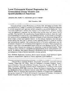
Figure 1: Plots of the relationship between square root of size measure (x1=2 i ) and estimated county total (t^i ) in selected counties at stage one for wind erosion (WEQ) and water erosion (USLE). Linear regression (REG1, REG2, REG3) and local linear regression (LPR1 with h = 3) ts are added in the plots.

REG3 LPR1(h=1) LPR1(h=3) LPR1(h=5)

2

4

6

8

10

12

8

10

12

sqrt(x)

0

USLE 10^6 2*10^6

REG3 LPR1(h=1) LPR1(h=3) LPR1(h=5)

2

4

6 sqrt(x)

Figure 2: Plots of the relationship between square root of size measure (x1=2 i ) and estimated county total (t^i ) in selected counties at stage one for wind erosion (WEQ) and water erosion (USLE). Linear regression (REG3) and local linear regression (LPR1 with h = 1; 3; 5) ts are added in the plots.

HT REG1 (x) / 1 REG2 (x) / x REG3 (x) / x2 LPR1 h=1 LPR1 h=3 LPR1 h=5

WEQ 443.6 (49.4) 485.9 (92.1) 448.7 (52.7) 442.5 (50.7) 434.1 (47.5) 427.4 (48.9) 430.5 (48.7)

USLE 551.5 (31.8) 544.4 (29.3) 540.2 (27.1) 537.8 (26.5) 529.0 (24.4) 532.3 (25.3) 541.2 (27.6)

Table 2: Horvitz-Thompson (HT), linear regression (REG1, REG2, REG3), and local linear regression (LPR1 with h = 1; 3; 5) estimates for wind erosion (WEQ) and water erosion (USLE) totals in millions of tons/acre/year. The numbers in parentheses are estimated standard errors. The Horvitz-Thompson (HT), linear regression (REG), and local linear regression (LPR1) estimates for WEQ and USLE totals and the corresponding variance estimates were calculated.1=2 We used the square root of the size measure xi instead of xi to reduce the sparseness of points in the regressor space. We calculated REG estimates with three different variances of the errors ((x) / 1; x; and x2 ), denoted by REG1, REG2, and REG3 respectively. This was done because the data displayed large amounts of heteroskedasticity (See Figure 1), aecting the parametric t. Three bandwidths (h = 1, 3, 5) were used for LPR1 (the smallest possible bandwidth to the nearest tenth for these data was h = 1). Figure 1 shows the relationship between square root of size measure (x1=2 i ) and estimated county total (t^i ) in counties selected at stage one for WEQ and USLE. Linear regression with three dierent error variances (REG1, REG2, REG3) and local linear regression with bandwidth h = 3 (LPR1(h = 3)) ts are added in the plots. In REG estimates, REG3, the best performing among them, has the smallest slope for both WEQ and USLE. The behavior of LPR1 is quite dierent from that of REG estimates in the sparse part of xi . Figure 2 shows the linear regression with the variance of the errors proportional to x2 (REG3) and local linear regression with three dierent bandwidths: LPR1(h = 1), LPR1(h = 3), and LPR1(h = 5).

Table 2 shows HT, REG and LPR1 estimates of WEQ and USLE totals and estimated standard errors. Using the estimated standard error as a guide, LPR1 with h = 1 performs best among all estimates and REG3 (REG with the variance of the errors proportional to x2 ) is best among REG estimates. Overall, LPR1 estimates except of the largest bandwidth are better than HT and REG estimates on the basis of estimated standard errors for both WEQ and USLE. In WEQ, the estimated standard error of REG is unexpectedly large, compared to that of HT. This seems to be due to the presence of a few strata with zero estimated variance for the HT estimator.

Acknowledgements This work was supported in part by cooperative agreement 68{3A75{43 between the USDA Natural Resources Conservation Service and Iowa State University. Computing for the research was done with equipment purchased with funds provided by an NSF SCREMS grant award DMS 9707740.

References Breidt, F.J. and Fuller, W.A. (1999) Design of supplemented panel surveys with application to the National Resources Inventory. Journal of Agricultural, Biological, and Environmental Statistics 4, 391{403.

Breidt, F.J. and Opsomer, J.D. (2000) Local polynomial regression estimators in survey sampling. Annals of Statistics, to appear. Chambers, R.L., Dorfman, A.H., and Wehrly, T.E. (1993). Bias robust estimation in nite populations using nonparametric calibration. Journal of the American Statistical Association 88, 268{277. Cochran, W.G. (1977). Sampling Techniques, 3rd ed. Wiley, New York. Dorfman, A.H. (1992). Nonparametric regression for estimating totals in nite populations. Proceedings of the Section on Survey Research Methods,

American Statistical Association, 622{625. Horvitz, D.G. and D.J. Thompson. (1952). A generalization of sampling without replacement from a nite universe. Journal of the American Statistical Association 47, 663{685. Sarndal, C.-E., Swensson, B., and Wretman, J. (1992). Model Assisted Survey Sampling, Springer, New York. Wand, M.P. and Jones, M.C. (1995). Kernel Smoothing, Chapman and Hall, London.