1.1.1 Starshaped unbiased estimates and the ix topology ..... other) nor its standard deviation is a constant (estimation neighborhoods are adaptive), as shown in ...
A novel anisotropic local polynomial estimator based on directional multiscale optimizations Alessandro Foi!∗ , Vladimir Katkovnik∗ , Karen Egiazarian∗ and Jaakko Astola∗ ∗ Institute of Signal Processing, Tampere University of Technology, Finland ! Dipartimento di Matematica, Politecnico di Milano, Italy
Abstract A novel anisotropic estimator for image restoration is presented. The proposed approach originates from the geometric idea of a starshaped estimation neighborhood topology. In this perspective, an optimal adaptation is achieved by selecting in a pointwise fashion the ideal starshaped neighborhood for the estimation point. In practice, this neighborhood is approximated by a sectorial structure composed by conical sectors of adaptive size. Special varying-scale kernels, supported on these sectors, are exploited in order to bring the original geometrical problem to a practical multiscale optimization. It is proposed to use this adaptive estimator iteratively. This recursion results in the anisotropic enlargement of the estimation neighborhood, an effect that can be interpreted as a special diffusion process. The resulting estimators are truly anisotropic, providing clean and accurate edge adaptation and excellent restoration performance. Their implementation is fast as it is based on simple convolutions and scalar optimizations. Although we focus on image processing, the approach is general and can be extended to higher-dimensional data. 1. Motivation and idea We consider the denoising problem of restoration of the image intensity y from the noisy observations z(x) = y(x) + σ η(x), η ∼ N (0, 1). Our main intention is to develop algorithms efÞcient for highly anisotropic images. When estimating y, a trade-off between noise suppression (variance) and smoothing (bias) has to be considered. Usual images are nonstationary, often characterized by localized features. Therefore, images should be treated adaptively: for example, one would achieve a higher noise suppression where the original image is smooth than in the vicinity of sharp transitions such as edges, where oversmoothing should be avoided. So, the desired balance between variance and bias depends on the image’s local features. How to control this balance is a key problem in adaptive signal processing. A novel strategy to achieve such adaptation is presented in this paper. 1.1 Estimates with support optimization kernel estimator (Þlter) in the form Let X ⊂ R2 (or ⊂ Z2 ) be the image! domain. Consider a conventional ! ! yˆ (x) =
1Ux (x − v)z(v)dv =
1U˜ x (v)z(v)dv =
z(v)dv/µ (Ux ) ,
(1.1)
U˜ x 1Ux has
where Ux is a neighborhood of the origin, and the uniform smoothing kernel support Ux and constant value 1/µ(Ux ) on Ux (µ(Ux ) stands for the Lebesgue measure of Ux ). We use the decoration ∼ to denote the translated and mirrored neighborhood about the reference point x, U˜ x (·) = Ux (x − ·), distinguishing it from Ux that is always about the origin. The term neighborhood (of a point) is used in a generic sense, meaning a simply connected set (containing the point). Relations between sets are always considered up to a null-set. " Bias and variance of the estimate (1.1) are, respectively, m yˆ (x) = y(x) − 1U˜ x (v)y(v)dv and σ 2yˆ (x) = σ 2 /µ (Ux ). The ideal support Ux∗ , yielding the best mean squared error, can be found by minimization of the quadratic risk l yˆ (x): l yˆ (x) = m 2yˆ (x) + σ 2yˆ (x). (1.2) Ux∗ = arg min l yˆ (x), U x " Thus yˆ (x) = 1Ux∗ (x − v)z(v)dv is the best local mean estimate of y (x). The optimization (1.2) can be quite difÞcult to achieve. In order to make it practical further speciÞcations of the problem are required. 1.1.1 Starshaped unbiased estimates and the Ux topology We discuss here a simpliÞed model, which will serve as a ground for the development of a more general approach. Let y be a binary black-and-white image, i.e. y (x) ∈ {0, 1} ∀x, and let us restrict our attention to starshaped unbiased estimates. It means that we consider only sets Ux which are starshaped with respect to the origin and such that m yˆ (x) = 0. The best estimate is obtained by minimization of the variance only or, equivalently, by maximization (with respect to the set inclusion ⊂) of the set Ux . Unbiasedness holds if and only if y (v) = y (x) for almost every v ∈ U˜ x . Under mild regularity assumptions on y (e.g. piecewise regular boundary of level sets), such equality has to hold for every v ∈ U˜ x . Thus, the best unbiased estimate corresponds to the largest starshaped Ux such that y(U˜ x (v)) = y (x) ∀v. This procedure can be formalized nicely in a topological manner. Let Ux be the topology constituted by all sets Ux such that: (i) Ux \ {0} is an open set in the Euclidean topology, (ii) Ux is starshaped with respect to 0 and (iii) y(x − v) = y (x) ∀v ∈ Ux . The maximum (w.r.t. ⊂) element in Ux corresponds to the ideal starshaped unbiased estimate of y (x), Ux∗ = max Ux . This suggests a risk minimization strategy based on a progressive set enlargement within this topology. It may be achieved also by “decomposing” Ux as follows. K be a collection of K starshaped neighborhoods of the origin such that ∪ K S = R2 (e.g. a collection of conical Let {Si }i=1 i =1 i S S K max U Si . It means that the sectors). Then, Uxi = {Ux i = Ux ∩ Si : Ux ∈ Ux } are also topologies, and Ux∗ = max Ux = ∪i=1 x S optimization can be performed independently on each “subcomponent” Uxi . Examples of the ideal U˜ x∗ are given in Figure 1 for two images: the characteristic function of an open disc and the “Cheese” image. Although different points x 2 , x 22 may
Figure 1: Examples of the ideal starshaped neighborhoods U˜ x∗ resulting from Ux∗ = max Ux .
Figure 2: Piecewise constant approximation of r ∗ (θ) and its representation by varying size sectors (a-b-c); adaptive fusing of uniform sectorial kernels gh ∗ (x,θ i ),θ i produces the equivalent uniform anisotropic kernel gx∗ (d-e). have U˜ x∗2 = U˜ x∗22 , the corresponding Ux∗2 and Ux∗22 are not equal, and in both examples each point x has its own different ideal neighborhood Ux∗ . Adapting perfectly to the edges, they are typically non-convex and their shape can be rather complex. Despite the apparent simplicity of these speculations, the practical realization of this approach can be still hard to achieve, since the function y is usually unknown and only its noisy observation z is available. In particular, unless y is known to belong to some very speciÞc class, ensuring unbiasedness is not possible, and biased estimates have to be considered. 1.2 Estimates with kernel scale optimization Another way to adapt to the signal’s varying local features, following the majority of multiscale techniques, is to "use kernels equipped with a scale parameter h (e.g. gh (·) = g(·/ h)/h 2 ). This estimate can be presented in the form yˆ (x) = gh(x) (x − v)z(v)dv. The scale optimization can be formulated, similarly to (1.2), as h ∗(x) = arg minh l yˆ . The bias and variance are, " " 2 respectively, m yˆ (x) = y(x) − gh(x) (x − v)y(v)dv, and σ 2yˆ (x) = σ 2 gh(x) (v)dv. This kind of optimization is known to be practical and can give good results through algorithms of reasonable complexity (e.g. Mallat, 1999). When the support of the kernel gh is bounded, the scale parameter h(x) controls the size of the neighborhood for estimation at the point x. The support of the optimal scale kernel gh ∗(x) can be thought as an approximation of the optimal Ux∗ considered in (1.2). However, traditional kernels have supports of simple convex geometry (square, rectangle, circle, oval, etc.) whereas the optimal neighborhoods can be quite complex, especially near edges or corners. Thus, this approximation of Ux∗ can be quite poor. 2. Anisotropic estimator based on adaptive directional scale A reasonable compromise between the geometrical approach discussed in section 1.1 and the above kernel-based method, is obtained with a directional adaptive scale estimator (Katkovnik et al., 2004). The considerations from section 1.1.1 shed some insight on how this sort of compromise is produced and clarify the geometrical properties of the estimator. The starshapedness of Ux∗ allows to describe this set using polar coordinates: there exists a function r ∗ (θ), θ ∈ [0, 2π) (see Figure 2a), such that Ux∗ = {v ∈ X, v = (v 1 , v 2 ) = (rv cos θ v ,rv sin θ v ) : rv < r ∗ (θ v )}. Instinctively, one may assume some sort of continuity of r ∗ (θ) with respect to its argument. This regularity, however, fails in the vicinity of edges where, as in the examples shown in Figure 1, r ∗ (θ) presents sharp transitions. This irregular behaviour is a direct manifestation of the anisotropy of y or, roughly speaking, that the function’s properties are different in different directions. The most natural model, allowing good approximation of such rapid transitions and also discontinuities is to assume r ∗ (θ) as a piecewise constant function of its angular argument, i.e. assuming that the optimal neighborhood Ux∗ has a sectorial structure, as shown in Figure 2(b-c). In our approach we exploit this sectorial decomposition. A collection of directional LPA (local polynomial approximation, see Fan & Gijbels, 1996) kernels {gh,θ i }h∈H,i=1,...,K supported on such sectors is designed. Each kernel is characterized by a direction θ k and a scale parameter h. The corresponding estimate is the convolution yˆh,θ i (x) = (gh,θ i ~ z) (x). The statistical ICI rule (Goldenshluger & Nemirovski, 1997; Katkovnik, 1999) is used to select a pointwise optimal scale h ∗ (x, θ i ) ≈ r ∗ (θ i ) for each direction. Let yˆh ∗(x,θ i ),θ i (x) be the directional optimal scale estimate and σ i2 (x) its variance. All these estimates can be fused in the Þnal one as follows: # # yˆ (x) = i λ(x, θ i ) yˆh ∗(x,θ i ),θ i (x), λ(x, θ i ) = σ i−2 (x)/ σ −2 (x). (2.1) j j The weights λ(x, θ i ) in the above convex combination are data-driven adaptive, as σ i−2 (x)" depend on the adaptive ∗ h ∗ (x, θ$ i ). The estimate (2.1) is equivalent to the adaptive anisotropic kernel estimate yˆ (x) = gx (x − v) z (v) dv, where ∗ ∗ gx = i λ(x, θ i )gh (x,θ i ),θ i . When uniform kernels gh,θ k are used, the adaptive weights λ(x, θ i ) make so that also the anisotropic kernel gx∗ is uniform on its support, i.e. gx∗ = 1∪i supp gh∗(x,θ ),θ , as shown in Figure 2(d-e). i i Figure 3 shows the estimation neighborhoods resulting from the proposed anisotropic LPA-ICI approach for noisy images (σ = 0.1). A comparison with Figure 1 shows the similarity between the previous ideal example and this concrete case.
Figure 3: “Cheese” and Cameraman (detail): optimal estimation neighborhoods U˜ x∗ obtained by ICI using sectorial kernels.
Figure 4: Recursive LPA-ICI: estimation neighborhood’s fattening (left), and layout of algorithm’s implementation (right). 2.1 Recursive LPA-ICI Þltering The idea behind this procedure is to apply recursively the anisotropic LPA-ICI algorithm, Þltering the Þnal output yˆ (2.1) once or many times over again. Denoting by LI the overall anisotropic LPA-ICI Þlter, this recursion is expressed as follows: z (1) = z, yˆ (l) = LI(z (l) ), z (l+1) = yˆ (l) , l = 1, 2, . . . . (2.2) (l) Expanding (2.2), in order to explicitly write y ˆ with respect to the initial observations z, we obtain ( ! ! %! ! & ' ∗(l−1) ∗(1) ··· g˜ x∗(l)(v (1) )g˜v (1) (v (2) )··· g˜ v (l−1)(v (l) ) dv (1)...dv (l−1) z(v (l) )dv (l) , (2.3) yˆ (l) (x) = gx∗(l) (x − v) yˆ (l−1) (v)dv = ∗(l)
where gx
∗(l)
is the anisotropic kernel at the l-th iteration, g˜ x
∗(l)
(·) = gx
(x − ·), and v (i) are auxiliary variables.
2.1.1 Estimation neighborhood’s enlargement Under the simple settings discussed in section 1.1.1, the ideal Ux∗ does not depend on the observed signal z, but rather only on the (unknown) signal y. When a second iteration is performed in (2.2), the ideal neighborhood for estimating y (x) from z (2) = yˆ (1) is again the same Ux∗ as in the Þrst iteration. Since this applies to all iterations, the whole process is described by replacing all kernels g˜ t∗(·) with 1U˜ ∗ in (2.3). Despite the ideal neighborhood Ux∗ is always the same for all t
l, the support of the resulting kernel that is used for integration against z(v (l) ) in the right hand side of (2.3) may grow at every " iteration. For example, at the second iteration the estimation support with respect to the initial observations z is supp 1U˜ ∗ (v)1U˜ ∗ (·)dv = ∪v∈U˜ ∗ U˜ v∗ . This is illustrated in Figure 4(left), with (a) some ideal starshaped neighborhoods U˜ v∗ x v x corresponding to points v belonging to, (b) the ideal neighborhood U˜ x∗ of the estimation point x, and (c) the resulting enlarged neighborhood of x, ∪ ˜ ∗ U˜ v∗ , obtained by the second iteration of the adaptive algorithm. Such sets are not necessarily v∈Ux
starshaped w.r.t. x. If the ideal neighborhoods were translation-invariant, Ux∗ = U ∗ ∀x, then (2.3) would take the simple convolutional form (l) yˆ (x) = (1U ∗ ~ · · · ~ 1U ∗ ~ z) (x), where convolution between kernels is repeated l-1 times. This resembles other iterative constructions, such as the Gaussian/Laplacian pyramids or wavelet-type projections (e.g. Mallat, 1999), where multiscale Þltering is obtained by recursively convolving the observations against the same Þlter. In general, however, formula (2.3) cannot be written in a simple convolutional form, because the adaptive kernels are not translation-invariant. Nevertheless, the considerations previously given about the enlargement of ideal neighborhoods hold similarly for the supports of the fused kernels. This anisotropic propagation of estimation neighborhoods realizes a diffusion ßow similar to the non-linear anisotropic diffusion (Perona & Malik, 1990), but intrinsically robust to noise because of the ICI-based adaptive scale. Regardless of their linear appearance, (2.3), as well as (2.1), are also non-linear estimators. The non-linearity is introduced by the adaptive selection of the directional scale h ∗(x, θ i ). 2.1.2 Variance of l-th iteration’s estimates " " ∗(1) (1) ∗(l−1) (2) (1) (l−1) , then, the standard deviation of the estimate Let G (l) x,h,θ i (·) = ··· (gh,θ i (x − v )g˜ v (1) (v )··· g˜ v (l−1) (·))dv ...dv
(l) (l) yˆh,θ (x), needed in order to use the ICI rule to select the optimal scale h ∗ (x, θ i ) at the l-th iteration, is σ ||G x,h,θ i ||2 . However, i its calculation is computationally quite complex, and it requires also a good deal of computer memory. These technical reasons limit the direct and accurate implementation of the recursive system (2.2). It would be appealing to use a simpler construction, where each step is performed without keeping track of the previous iterations, i.e. using the LI operator as a “black box”, with a pair of inputs (observations and their standard deviations) and a pair of outputs (estimates and their standard deviations), as shown in Figure 4(right).
Figure 5: Fragment of the Cameraman image: from left to right, original, noisy image, LPA-ICI estimate (Þrst iteration), recursive LPA-ICI estimate (second iteration). Further iterations of the recursive procedure yield visually identical estimates. 2.1.3 Implementation The residual noise in the estimate yˆ from (2.1) is no longer uncorrelated (estimation neighborhoods may overlap with each other) nor its standard deviation is a constant (estimation neighborhoods are adaptive), as shown in Figure 4(right). The $ expression for its variance is σˆ y2ˆ (x) = 1/ i σ −2 i (x). If we assume that this residual noise is uncorrelated, the standard (2) deviation of the directional estimates yˆh,θ (x) for the second stage of the recursive algorithm would be simply calculated i
2 ~ σˆ 2 )1/2 , avoiding the use of the complicated kernel G (2) . This reasoning may be extended to as the convolution (gh,θ x,h,θ i yˆ (1) i further iterations, assuming that the noise in yˆ (l) is always uncorrelated. However, as this assumption does not hold, the quality of estimation deteriorates, and typically results in oversmoothing of details in the image. It turns out, for low-order kernels, that a simple compensating factor for the standard deviation can effectively reduce this degeneration. This modiÞcation of the calculation of the variance may be interpreted as an attempt to Þlter out only the white component of the residual noise. After setting the initial conditions y (0) = z and σˆ y(0) ≡ σ , the l-th recursive step of the modiÞed recursive algorithm is %# & ' (−1/2 (l) −2 yˆ (l) = LI( yˆ (l−1) ), σ ˆ σˆ yˆ (l) = , l = 1, 2, . . . , i i (l)
where σˆ i = σˆ yˆ (l)
h ∗(x,θ i ),θ i
2 ~ σˆ 2 1/2 , σˆ yˆ (l) = α(gh,θ yˆ (l−1) ) , and α < 1 being the Þxed correcting factor. i h,θ i
In spite of the striking simplicity of the modiÞcation, simulation results show that it enables ICI to properly select the adaptive scale. Moreover, convergence of the above recursive system is easily guaranteed, since σˆ (l) = O(αl ) → 0. More yˆ
≤ cαl σ . This implies that yˆ (l) (x) precisely, since ||gx∗ ||2 ≤ 1, there exist a constant c such that | yˆ (l) (x) − yˆ (l+1) (x) | < cσˆ y(l) ˆ (x) ) * is a Cauchy sequence. Qualitatively, the actual convergence rate of the algorithm depends on µ Ux∗ ≈ ||gx∗ ||−1 2 , and usually the algorithm reaches a numerical steady-state already after three iterations. The proposed recursive method can be used for accurate detail-preserving image denoising, segmentation and edge detection applications. Table 1 shows the ISNR and MAE (/1-distance) results for the restoration of the Cameraman image, corrupted by additive Gaussian white noise, σ = 0.1. Zero-order uniform kernels for a total of eight directions and four scales, h ∈ {1, 2, 3, 5}, were used with Þxed α = 2/3. These results are illustrated (for a fragment of the image) in Figure 5. The table shows a fast convergence of the iterations and criteria values attesting the high quality of the Þltering. iteration # noisy 1 2 3 4 5 6 ISNR (dB) 0 7.361 8.098 8.119 8.120 8.120 8.120 255∗MAE 20.38 7.894 6.597 6.538 6.535 6.535 6.535 Table 1: ISNR and MAE results for the Cameraman image denoising experiment (σ =0.1, SNR=14.39dB). The use of higher order kernel mixtures, together with a more reÞned update of the standard deviations and a larger set of scales allows to achieve, for the same experiment, an ISNR of 7.50, 8.23 and 8.47dB at the Þrst, second and third iteration, respectively. A similar performance cannot be achieved by the non-recursive algorithm. References FAN , J. & G IJBELS , I. 1996. Local polynomial modelling and its application, Chapman and Hall, London. G OLDENSHLUGER , A. & N EMIROVSKI , A. 1997. On spatial adaptive estimation of nonparametric regression, Math. Meth. Statistics, 6, 135-170. K ATKOVNIK , V. 1999. A new method for varying adaptive bandwidth selection, IEEE Trans. on Signal Proc., 47(9), 2567-2571. K ATKOVNIK , V., E GIAZARIAN K., & A STOLA , J. 2002. Adaptive window size image de-noising based on intersection of conÞdence intervals (ICI) rule, J. of Mathematical Imaging and Vision, 16(3), 223-235. K ATKOVNIK , V., F OI , A., E GIAZARIAN , K., & A STOLA , J. 2004. Directional varying scale approximations for anisotropic signal processing, Proceedings of XII European Signal Processing Conference, EUSIPCO 2004, Vienna, Austria, 6-10 Sept. 2004, 101-104. M ALLAT, S., 1999. A wavelet tour of signal processing, second edition, Academic Press, New York. P ERONA , P., & M ALIK , J. 1990. Scale-space and edge detection using anisotropic diffusion, IEEE Transactions on Pattern Analysis and Machine Intelligence, 12(7), 629-639.