Long Range Parametric Channel Prediction for ... - CiteSeerX

Long Range Parametric Channel Prediction for Narrowband MIMO Systems with Joint Parameter Estimation Ramoni O. Adeogun, Paul D. Teal and Pawel A. Dmochowski School of Engineering and Computer Science Victoria University of Wellington, Wellington New Zealand E-mail:{ramoni.adeogun,paul.teal,pawel.dmochowski}@ecs.vuw.ac.nz

Abstract—In this paper, we propose a novel long range prediction scheme for narrowband MIMO systems using realistic spatial channel model. The algorithm exploits both the temporal and spatial structure of the MIMO channel to jointly estimate the multipath parameters via a subspace based three dimensional ESPRIT approach. We propose simple transformations to convert the channel impulse response into a space-time manifold matrix exhibiting translational invariance in three dimensions. Simulation results show that the proposed prediction scheme outperforms existing algorithms and can achieve prediction range of several wavelengths. Index Terms—Channel prediction, MIMO, parameter estimation, ESPRIT, multipath propagation, spatial channel model.

I. I NTRODUCTION Provision of high data rates and quality of service with increased reliability for an increasing number of users constitute a major challenge facing current and future wireless communication systems. In order to meet these stringent requirements, adaptive and limited feedback based multiple input multiple output (MIMO) transmission techniques have been chosen as a key scheme in recent and future wireless standards such as IEEE 802.11n, Long Term Evolution (LTE) and LTE-Advanced due to the possibility of adapting transmission parameters based on the channel state information (CSI). These schemes however require both the transmitter and receiver to have knowledge of the CSI. In frequency division duplexing systems, channel state information at the transmitter is often acquired by estimation at the receiver and feedback to the transmitter [1]. Delays in the feedback link, however, make the CSI outdated before usage at the transmitter. Long range prediction is therefore required in order to mitigate performance loss. CSI prediction for single input single output (SISO) systems has been well addressed in literature and have been shown to offer significant improvement in system performance (see e.g [2]–[5]). Channel prediction for MIMO systems has also received considerable research attention within the last decade. The possibility of predicting multi-antenna channels was first investigated in [6]. It was shown that channel prediction improves MISO smart antenna system performance. In [7], linear prediction scheme for the direct prediction of precoding and

decoding vectors using geodesic interpolation was proposed for narrowband MIMO systems. Similar prediction algorithms exploiting geodesic interpolation and parallel transport for the prediction of channel direction in codebook based MIMO systems have been proposed in [8]. These schemes however assumed that the MIMO channel is independent and identically distributed without account for the propagation phenomenon. Bounds on the prediction error of MIMO channels [9] indicate that better prediction can be obtained by utilizing the spatial parameters of the MIMO channel. The authors used autoregressive ( AR) modelling for the prediction of a beamspace transformed CSI and an inverse transformation was performed on the predicted CSI. The proposed beamspace transformation matrix is, however, not well conditioned and so the inverse transformation is difficult to perform. A similar approach based on ray cancelling was presented in [10]. The scheme utilizes QR decomposition to overcome the ill-conditioning of the transformation matrix. It was however assumed that the angles of arrival and angles of departure are known. In [11], the ESPRIT based scheme for single input single output system proposed in [2] was extended to the prediction of MIMO channels. This approach is not optimal since it does not utilize the spatial information. It was also shown in [9] that parametric predictors based on the double directional MIMO model are likely to achieve optimal performance. In [12], the possibility of exploiting spatial structure of MIMO channel in enhancing prediction using multichannel linear prediction was studied. The authors showed using both synthesized and measured data that multichannel linear prediction is unreliable for MIMO channel with dense scattering. In [13], we proposed a prediction algorithm for narrowband MIMO channel that exploits the receive spatial and temporal correlations in realistic spatial channel models. The predictor utilizes a transmit spatial signature model (TSS) based on the assumption that the dependence of transmit steering vectors on angle of arrival can be removed due to the stationarity of the transmitter. Although, the performance of the proposed algorithm was shown to be better than previous method, the transmitter spatial information is not utilized for the prediction. Motivated by the benefits of using CSI prediction with

adaptive and limited feedback MIMO schemes and the need for efficient low complexity multidimensional parameter estimation schemes to enhance MIMO CSI prediction [9], we make the following contributions in this paper ∙ We propose a simple and efficient scheme for transforming samples of the MIMO channel impulse response into a data matrix equivalent to having a 3D array with certain invariance structure. The transformation allow for efficient utilization of both the temporal and spatial structure of the channel. ∙ We propose an ESPRIT based scheme for jointly estimating the AOAs, AODs, and Doppler shifts in narrowband MIMO systems. ∙ We study the prediction of narrowband MIMO systems using the double directional spatial model with the proposed parameter estimation scheme. We further perform simulations to evaluate the performance of the algorithm. The rest of this paper is organized as follows. In section II, we describe the spatial channel model (SCM) upon which the prediction scheme is based along with a data transformation approach. The proposed prediction algorithm is presented in section III. Section IV presents the simulation set-up along with results and discussions. Finally, we present the conclusion in V. II. M ODELS In this section, we present a description of the narrowband double directional MIMO model along with the proposed transformations and a derivation of the data model. A. Channel Model A commonly used multipath channel model is the ray based sum of sinusoids model, defined for a single input single output (SISO) system as the superposition of 𝑃 scattering sources [14] 𝑃 (𝑡)

ℎ(𝑡) =

∑

𝛼𝑝 (𝑡) exp(𝑗𝜔𝑝 𝑡)

(1)

𝑝=1

where 𝛼𝑝 is the complex amplitude of the 𝑝th scattering source and 𝜔𝑝 is the Doppler frequency defined as 𝜔𝑝 = 𝜅𝑉 cos 𝜃𝑝 (𝑡)

(2)

where 𝑉 is the mobile velocity, 𝜃𝑝 (𝑡) is the angle of arrival of the 𝑝th scatterer relative to the mobile station direction, 𝜅 = 2𝜋 𝜆 is the wave number and 𝜆 is the wavelength. The SISO model in (1) can be extended to modelling of a MIMO propagation channel via the introduction of the spatial dimension [9] 𝑃 (𝑡)

H(𝑡) =

∑

𝛼𝑝 (𝑡)b𝑟 (𝜃𝑝 (𝑡))b𝑇𝑡 (𝜙𝑝 (𝑡)) exp(𝑗𝜔𝑝 𝑡)

(3)

𝑝=1

where 𝜙𝑝 (𝑡) is the angle of departure and b𝑟 (𝜃𝑝 (𝑡)) and b𝑇𝑡 (𝜙𝑝 (𝑡)) are the receive and transmit array response vectors in the direction of the 𝑝th scattering source, respectively. For

a uniform linear array (ULA) aligned perpendicular to the direction of motion with antenna spacing Δ𝑟 at the receiver, the receive array steering vector is defined as b𝑟 (𝜃𝑝 ) = [1, exp(𝑗Ω𝑝 ), ⋅ ⋅ ⋅ , exp(𝑗(𝑁 − 1)Ω𝑝 )]𝑇

(4)

where Ω𝑝 = 2𝜋Δ𝑟 sin 𝜃𝑝 and 𝑁 is the number of receive antenna elements. The transmit response vector, b𝑡 (𝜙𝑝 ), is obtained by replacing Δ𝑟 with Δ𝑡, 𝜃𝑝 with 𝜙𝑝 and 𝑁 with 𝑀 in (4), where Δ𝑡 denotes the antenna separation at the transmitter. In order to reduce the problem of modelling the time varying MIMO channel to a classical parameter estimation problem, we assume that the multipath parameters remain constant over the region of interest1 and that the mobile velocity remains constant (such that constant temporal sampling corresponds to constant spatial sampling). The simplified sampled MIMO model is therefore H(𝑘) =

𝑃 ∑

𝛼𝑝 b𝑟 (𝜃𝑝 )b𝑇𝑡 (𝜙𝑝 ) exp(𝑗𝑘𝜈𝑝 )

(5)

𝑝=1

where 𝜈𝑝 = 𝜅𝑉 Δ𝑡 cos 𝜃𝑝 is the normalized Doppler shift of the 𝑝-th path and Δ𝑡 is the temporal sampling interval. B. Data Transformation Prediction of the MIMO channel using the model in (5) requires estimation of the multipath parameters 𝜸 = [𝜶, 𝜽, 𝝓, 𝝂]. We will now present a simple transformation to enable joint estimation of these parameters. Assuming there are 𝐾 available samples of the CSI from channel estimation or measurements, we perform the following vectorization operation on the samples h(𝑘) = vec [H(𝑘)] =

𝑃 ∑

𝑘 = 1, ⋅ ⋅ ⋅ , 𝐾

[ ] vec 𝛼𝑝 b𝑟 (𝜃𝑝 )b𝑡 (𝜙𝑝 )𝑇 exp(𝑗𝑘𝜈𝑝 )

(6)

𝑝=1

It can be easily shown that the vectorized channel transfer function in (6) can be modelled as h(𝑘) =

𝑃 ∑

𝛼𝑝 b𝑟 (𝜃𝑝 ) ⊗ b𝑡 (𝜙𝑝 ) exp(𝑗𝑘𝜈𝑝 )

(7)

𝑝=1

where ⊗ denotes the Kronecker product. We then form an 𝑁 𝑀 𝑄 × 𝑅 Hankel matrix from the vectorized channel as ⎤ ⎡ h(1) h(2) ⋅⋅⋅ h(𝑅) ⎢ h(2) h(3) ⋅ ⋅ ⋅ h(𝑅 + 1)⎥ ⎥ ⎢ ⎥ (8) ℋ=⎢ .. .. ⎥ ⎢ .. .. . ⎦ ⎣ . . . h(𝑄)

h(𝑄 + 1)

⋅⋅⋅

h(𝐾)

where 𝑄 denotes the number of temporal correlation lags and 𝑅 = (𝐾 − 𝑄 + 1) is the number of averages used in the 1 This multipath parameters stationarity assumption has been shown to be valid within the standardized WINNER/3GPP Spatial Channel Models (SCM) for as long as 50 𝜆 [15].

covariance computation. Let a𝑑 (𝜈) be a 𝑄-dimensional vector defined as a𝜄𝑑 (𝜈) = [exp(𝑗𝜄𝜈), exp(𝑗(𝜄 + 1)𝜈), ⋅ ⋅ ⋅ , exp(𝑗(𝑄𝜄 )𝜈)]

𝑇

(9)

where 𝑄𝜄 = 𝜄 + 𝑄 − 1. By using the transformations in (8) and the model in (7), the data in the 𝑠th column of ℋ can be expressed as ℋ𝑠 =

𝑃 ∑

SUBSPACE DIMENSION ESTIMATION

CHANNEL SIMULATOR

COVARIANCE MATRIX/EVD

JOINT AOA, AOD & DOPPLER EST.

COMPLEX AMPLITUDE ESTIMATION

CHANNEL PREDICTI ON

AWGN GENERATOR

𝛼𝑝 (b𝑟 (𝜃𝑝 ) ⊗ b𝑡 (𝜙𝑝 ) ⊗ a𝑠𝑑 (𝜈𝑝 )),

(10)

𝑝=1

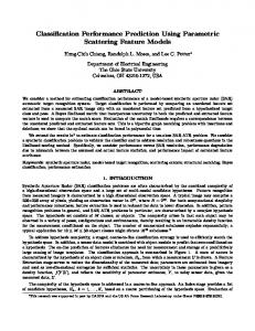
Fig. 1: Block diagram of the proposed ESPRIT based MIMO channel prediction scheme.

which has a compact representation ℋ𝑠 = B(𝜃, 𝜙, 𝜈)𝜶

(11)

where 𝜶 = [𝛼1 , 𝛼2 , ⋅ ⋅ ⋅ , 𝛼𝑃 ]𝑇 and B(𝜃, 𝜙, 𝜈) = [b𝑟 (𝜃1 ) ⊗ b𝑡 (𝜙1 ) ⊗ a𝑠𝑑 (𝜈1 ), ⋅ ⋅ ⋅ , b𝑟 (𝜃𝑃 ) ⊗ b𝑡 (𝜙𝑃 ) ⊗ a𝑠𝑑 (𝜈𝑃 )] is an 𝑁 𝑀 𝑄×𝑅 space-time manifold matrix. The model in (11) can be employed to jointly estimate the angle of arrival (AOA), angle of departure (AOD) and Doppler shifts. We next present the proposed MIMO channel prediction algorithm which we call Multidimensional ESPRIT based MIMO CHAnnel Predictor (MEMCHAP). III. MEMCHAP The proposed channel prediction algorithm comprises of two stages viz multipath parameter estimation and prediction. A. Parameter Estimation The multipath parameter estimation stage is divided into four sub-stages: Covariance Matrix Estimation, Subspace dimension estimation, Joint AOA, AOD and Doppler estimation and Amplitude Estimation. 1) Covariance Matrix Estimation: The parameter estimation stage depends on the singular value decomposition (SVD) of the Hankel matrix in (8) or the eigenvalue decomposition (EVD) of the spatio-temporal covariance matrix computed using ℋℋ𝐻 (12) Z= 𝑅 where [.]𝐻 denotes the Hermitian conjugate transpose. 2) Subspace Dimension Estimation: The number of sources is estimated using the Minimum Mean Squared Error (MMSE) based Minimum Description Length (MDL) criterion defined as [16] MMDL(𝑢) (13) 𝑃ˆ = arg min 𝑢=1,⋅⋅⋅ ,𝑈 −1

where 𝑈 = 𝑁 𝑀 𝑄 and MMDL(𝑢) is given by 1 MMDL(𝑢) = 𝑅 log(𝜆𝑢 ) + (𝑢2 + 𝑢) log 𝑅 2

3) Joint AOA, AOD and Doppler Estimation: Using the idea of translational invariance in ESPIRIT [17] and multiple invariance ESPRIT [18], [19], we derive a 3D algorithm to jointly estimate the AOA, AOD and Doppler shifts at this stage. We perform EVD or SVD of Z and decompose the eigenvectors into signal and noise subspace matrices. In order to explore the translational invariance structure in the spacetime manifold matrix, we defined the following 1D and 3D selection matrices ] [ J𝜃1 = I𝑀 ⊗ I𝑄 ⊗ J1𝜃 J1𝜃 = I(𝑁 −1) 0(N−1) ] [ J𝜃2 = I𝑀 ⊗ I𝑄 ⊗ J2𝜃 J2𝜃 = 0(𝑁 −1) I(N−1) ] [ J𝜙1 = I𝑄 ⊗ J1𝜑 ⊗ I𝑁 J1𝜙 = I(𝑀 −1) 0(M−1) ] [ J𝜙2 = I𝑄 ⊗ J2𝜙 ⊗ I𝑁 J2𝜙 = 0(𝑀 −1) I(M−1) ] [ J𝜈1 = J1𝜈 ⊗ I𝑁 ⊗ I𝑀 J1𝜈 = I(𝑄−1) 0(Q−1) ] [ J𝜙2 = J2𝜈 ⊗ I𝑁 ⊗ I𝑀 (15) J2𝜈 = 0(𝑄−1) I(Q−1) where I𝐿 is an 𝐿 × 𝐿 identity matrix and 0𝐿 ∈ R𝐿 is an Ldimensional vector of zeros. Using the 3D selection matrices in (15), we define the following invariance equations 𝐽𝜃2 ES = 𝐽𝜃1 E𝑆 Θ 𝐽𝜙2 ES = 𝐽𝜙1 E𝑆 Φ 𝐽𝜈2 ES = 𝐽𝜈1 E𝑆 N

(16)

where ES is the 𝑁 𝑀 𝑄× 𝑃ˆ signal subspace matrix having the eigenvectors corresponding to the 𝑃ˆ largest eigenvalues of Z as its columns. The matrices Θ, Φ and N are matrices whose eigenvalues contain information about the parameter, that is ] [ eig(Θ) = diag exp(𝑗2𝜋Δ𝑟 sin 𝜃1 ), ⋅ ⋅ ⋅ , exp(𝑗2𝜋Δ𝑟 sin 𝜃𝑃ˆ ) ] [ eig(Φ) = diag exp(𝑗2𝜋Δ𝑡 sin 𝜙1 ), ⋅ ⋅ ⋅ , exp(𝑗2𝜋Δ𝑡 sin 𝜙𝑃ˆ ) ] [ (17) eig(N) = diag exp(𝑗𝜈1 ), ⋅ ⋅ ⋅ , exp(𝑗𝜈𝑃ˆ ) where eig(.) denotes the eigenvalues of the associated matrix. Solutions to the equations in (16) are then obtained using the Least Square(LS) approach Θ = ((𝐽𝜃2 ES )𝐻 (𝐽𝜃2 ES ))−1 (𝐽𝜃2 ES )𝐻 (𝐽𝜃1 E𝑆 )

(14)

Φ = ((𝐽𝜙2 ES )𝐻 (𝐽𝜙2 ES ))−1 (𝐽𝜙2 ES )𝐻 (𝐽𝜙1 E𝑆 ) N = ((𝐽𝜈2 ES )𝐻 (𝐽𝜈2 ES ))−1 (𝐽𝜈2 ES )𝐻 (𝐽𝜈1 E𝑆 )

(18)

It should be noted that although estimates of the AOAs, AODs, and normalized Doppler shifts can be obtained directly from solutions of (18), this requires an additional algorithm to pair the estimates. However, automatic pairing of the estimates is achieved in this paper by using a scheme similar to the mean eigenvalue decomposition (MEVD) [20]. Denoting Y =Θ+Φ+N

(19)

TABLE I: Simulation Parameters Parameter Number of Drops (Realizations) Sampling Interval Mobile Speed Carrier frequency Number of Paths Transmit Antenna Array Receive Antenna Array Samples (Predictor initialization)

Value 1000 2ms 75 kmh−1 2.1 GHz 10 ULA (120 deg sectoral) ULA 100-500

We eigen-decompose Y to obtain the common eigenvectors of the three matrices in the sum Y = ΠΛΠ−1

(20)

The diagonal eigenvalue matrices are then computed using Z𝜃 = Π−1 ΘΠ Z𝜙 = Π−1 ΦΠ Z𝜈 = Π−1 NΠ

(21)

where Z𝜃 = eig(Θ), Z𝜙 = eig(Φ) and Z𝜈 = eig(N). Estimates of the parameters are then obtained from (17) as ( ) − angle(diag(Z𝜃 )) 𝜽 = asin 2𝜋Δ𝑟 ) ( − angle(diag(Z𝜙 )) 𝝓 = asin 2𝜋Δ𝑡 (22) 𝝂 = angle(diag(Z𝜈 )) 4) Amplitude Estimation: We assumed that the complex amplitude of each multipath is same far all antenna pairs and utilize the first entry of the MIMO channel matrix for the amplitude estimation. Owing to the Vandermode structure of the array steering matrix, the first entry of the MIMO matrix in (4) can be modelled as ℎ11 (𝑘) =

𝑃 ∑

𝛼𝑝 exp(𝑗(𝑘 − 1)𝜈𝑝 )

(23)

𝑝=1

The following sets of linear equations can therefore be formed using the 𝐾 available samples ⎤⎡ ⎤ ⎡ ⎤ ⎡ 1 1 ⋅⋅⋅ 1 𝛼1 ℎ11 (1) ⎥⎢ ⎥ ⎢ ℎ (2) ⎥ ⎢ 𝑔 𝑔 ⋅ ⋅ ⋅ 𝑔 ⎢ ⎥ ˆ 1 2 𝛼2 ⎥ 𝑃 ⎢ 11 ⎥ ⎢ ⎥⎢ ⎢ ⎢ ⎥ ⎥=⎢ . ⎥ . . .. .. ⎥ ⎢ .. ⎥ ⎢ . .. .. ⎥ ⎢ . ⎣ . ⎦ ⎣ . ⎦⎣ . ⎦ ℎ11 (𝐾)

(𝐾−1)

𝑔1

(𝐾−1)

𝑔2

⋅⋅⋅

(𝐾−1)

𝑔𝑃ˆ

𝛼𝑃ˆ

(24) The complex amplitudes are obtained via a solution of (24) as 𝜶 = (G𝐻 G)−1 G𝐻 h11 = G† h11 where (.)† denotes the Moore-penrose pseudoinverse.

(25)

B. Prediction Once we have estimated all parameters of the MIMO model in (3), prediction is achieved by substitution into the model for the desired horizon. The predicted MIMO impulse response is thus 𝑃 ∑ ˜ )= 𝛼 ˆ 𝑝 b𝑟 (𝜃ˆ𝑝 )b𝑇𝑡 (𝜙ˆ𝑝 ) exp(𝑗𝜏 𝜈ˆ𝑝 ) (26) H(𝜏 𝑝=1

where 𝜏 is the desired time instant. IV. N UMERICAL S IMULATIONS In the section, we evaluated the performance of the proposed predictor. The prediction performance is evaluated in terms of the normalised mean squared error (NMSE) defined as 1 ˜ 𝔼[∣∣H(𝑡) − H(𝑡)∣∣2𝐹 ] 𝑃𝐻 (𝜏 − 𝐾) 𝐿 𝜏 ∑ ∑ 1 ˜ ≈ ∣∣H(𝑡) − H(𝑡)∣∣2𝐹 𝐿𝑃𝐻 (𝜏 − 𝐾)

NMSE(𝜏 ) =

ℓ=1 𝑡=𝐾+1

(27) where [.]𝐹 denotes the Frobenious norm, 𝐿 is the number of realizations and 𝑃𝐻 denotes the power of the MIMO channel defined as 𝐾+𝐾𝑝 ∑ 1 ∣∣H∣∣2𝐹 (28) 𝑃𝐻 = 𝐾 + 𝐾𝑝 𝑡=1 where 𝐾𝑝 denotes the overall prediction horizon considered. The predictions were performed using the parameters in Table I except where stated otherwise. The channel is generated using the double directional MIMO model with uniformly distributed AOAs (∼ 𝑈 [0, 2𝜋)) and AODs (∼ 𝑈 [− 𝜋3 , 𝜋3 )) and Gaussian distributed complex amplitudes (∼ 𝒩 (0, 1)). Since outdoor environments are dominated by a small number of multipath components with relatively large power, we used the number of paths 𝑃 = 10 [6] for our simulations. In order to model measurement/estimation noise and multiuser interference, we added temporally and spatially white complex Gaussian noise to the channel. A 2x2 MIMO system is considered for the simulations except where otherwise stated. We plot the trace of amplitudes of the actual and predicted CSI at 𝑆𝑁 𝑅 = 10 𝑑𝐵 in Fig. 2 where the horizontal axis denotes time in seconds. Clearly, the proposed algorithm can accurately track the time varying channel for both observation and prediction region. The AR prediction scheme however,

15

AR

−2

10

−3

10

0

0.1

0.2

0.3

0.4

0.5 0.6 Prediction Time (s)

MEMCHAP SNR=0dB MEMCHAP SNR=5dB MEMCHAP SNR=15dB AR PREDICTION SNR=0dB AR PREDICTION SNR=5dB AR PREDICTION SNR=15dB 0.7 0.8 0.9 1

Fig. 3: Channel Prediction NMSE versus time. Prediction initialized with training length of 400 samples

15 MEMCHAP

True Channel

10 H12

H11

−1

10

NMSE

loses track of the channel after a short prediction interval. In Fig. 3, we present the normalized mean square error (NMSE) for the proposed algorithm and AR prediction at 𝑆𝑁 𝑅 = [0, 5, 15] 𝑑𝐵. It can be seen from the figure that the proposed scheme outperforms the AR-based predictor at all noise levels. In Fig. 4, we plot the NMSE of the proposed predictor initialized with different number of samples. As can be seen in the figure, increasing the training length improves the prediction performance. This is expected since better parameter estimation performance is achieved with increased number of samples. The CDF of prediction NMSE for a prediction interval of 10 ms (≈ 1.5 𝜆) at different noise level is shown in Fig. 5. In Fig 6, we present the CDF of prediction NMSE for a prediction interval of 50 ms (≈ 7.5 𝑙𝑎𝑚𝑏𝑑𝑎) at different SNR levels. As shown in the figure, the performance of the algorithm is still acceptable for such a long prediction range.

10

5

5

0 0.9

0 0.9

−1

10 1

1.05 1.1 Time(s)

1.15

0.95

1

1.05 1.1 Time(s)

1.15

1.2 NMSE

0.95

15 10

−2

10

H21

H22

10 0

5

MEMCHAP 200 Samples MEMCHAP 300 Samples MEMCHAP 400 Samples MEMCHAP 500 Samples

−10 0 0.9

0.95

1

1.05 1.1 Time(s)

1.15

0.9

0.95

1

1.05 1.1 Time(s)

1.15

1.2

Fig. 2: 2x2 MIMO Channel Trace at SNR = 10 dB. Prediction initialized with training length of 500 samples

−3

10

R EFERENCES [1] D. J. Love, R. W. Heath-Jr., V. K. N. Lau, D. Gesbert, B. D. Rao, and M. Andrews, “An overview of limited feedback in wireless communi-

0.1

0.2

0.3

0.4

0.5 0.6 Prediction Time(s)

0.7

0.8

0.9

1

Fig. 4: Channel Prediction NMSE versus time at SNR = 5 dB

V. C ONCLUSION We proposed a novel algorithm for the long range prediction of time-varying narrowband MIMO channels. The multipath channel is described by the double directional multi-antenna model with angle of arrival, angle of departure, Doppler shifts and complex amplitude parameters which are jointly estimated through a three dimensional ESPRIT based algorithm and the channel is then predicted using these parameters which are assumed stationary over the region of interest. Simulation results shows that the proposed algorithm can effectively extrapolate the channel into the future even at low signal to noise ratio. Future work will analyse the performance of the proposed algorithm in terms of the overall system performance metrics and on measured data.

0

[2]

[3]

[4]

[5]

[6]

[7]

[8]

cation systems,” IEEE Journal on Selected Areas in Communications, vol. 26, no. 8, pp. 1341–1365, 2008. J. Andersen, J. Jensen, S. Jensen, and F. Frederisen, “Prediction of future fading based on past measurements,” in IEEE Vehicular Technology Conference, vol. 1, 1999, pp. 151–155. P. Teal and R. Vaughan, “Simulation and performance bounds for realtime prediction of the mobile multipath channel,” in IEEE Workshop on Statistical Signal Processing Proceedings, 2001, pp. 548–551. A. Duel-Hallen, S. Hu, and H. Hallen, “Long Range Prediction of Fading Signals: Enabling Adaptive Transmission for Mobile Radio Channels,” IEEE Sig. Proc. Magazine, vol. 17, pp. 62–75, 2000. A. Duel-Hallen, “Fading Channel Prediction for Mobile Radio Adaptive Transmission Systems,” Proceedings of the IEEE, vol. 95, no. 12, pp. 2299–2313, 2007. A. Arredondo, K. R. Dandekar, and G. Xu, “Vector channel modeling and prediction for the improvement of downlink received power,” IEEE Trans. on Comm., vol. 50, no. 7, pp. 1121–1129, 2002. H. T. Nguyen, J. B. Andersen, and G. F. Pedersen, “Capacity and performance of MIMO systems under the impact of feedback delay,” in PIMRC, 2004, pp. 53–57. J. Chang, I.-T. Lu, and Y. Li, “Adaptive Codebook Based Channel Prediction and Interpolation for Multiuser MIMO-OFDM Systems,” in ICC, 2011, pp. 1–5.

1 0.9

CDF(Pr(NMSE