Zukang Shen, Jeffrey G. Andrews, and Brian L. Evans. Wireless Networking and Communications Group. Department of Electrical and Computer Engineering.
Short Range Wireless Channel Prediction Using Local Information Zukang Shen, Jeffrey G. Andrews, and Brian L. Evans Wireless Networking and Communications Group Department of Electrical and Computer Engineering The University of Texas at Austin, Austin, Texas 78712 Email: {shen, jandrews, bevans}@ece.utexas.edu
Abstract— Wireless channels change due to the mobility of users, which coupled with system delays, causes outdated channel state information (CSI) to be used for transmitter optimization techniques such as adaptive modulation. Channel prediction allows the system to adapt modulation methods to an estimated future CSI. The primary contribution of this paper is a low complexity channel prediction method using polynomial approximation. The method is local in the sense that only a few previous channel samples are required to estimate the next CSI. The computational complexity of the proposed method is demonstrated to be negligible compared to previous methods. Simulation results show that the proposed method accurately tracks slowly to moderately fading channels. The proposed method’s usefulness is demonstrated by applying it to a multiuser OFDM system. As an example, a multiuser OFDM with a system delay of 5 ms and a Doppler spread of 40 Hz loses about 17% of its capacity due to imperfect CSI. Using the proposed algorithm to predict the CSI, the capacity loss is less than 1%.
I. I NTRODUCTION Adaptive modulation [1] uses different signal constellations to different channel conditions to increase spectrum efficiency. Recently multiuser orthogonal frequency division multiplexing (MU-OFDM) [2]-[5] is gaining interest. By allocating subchannels and power adaptively based on channel conditions, MU-OFDM can achieve much higher capacity compared to fixed resource allocation schemes, such as fixed TDMA or FDMA. However, knowledge of instantaneous channel condition is required to determine the resource allocation. Due to various delays, such as transmission, hardware, and computational delays, the computed schemes may not be optimal with respect to the current channel condition, and thus may degrade the system performance. If channel state information (CSI) could be reliably predicted, then the subchannels and power could be allocated for future conditions. Researchers have realized the importance of channel prediction and various channel estimation algorithms have been proposed [6]. In [7], a deterministic channel model is proposed to perform short range channel prediction. The channel is modelled as a composite signal with tens of incident waves, whose amplitudes, frequencies, and phases are slowly varying. Spectrum estimation algorithms, such as the Multiple Signal Classification algorithm and the minimum norm algorithm, have been applied to estimate the parameters of incident waves. In [8], CSIs are predicted by an auto-regressive model, followed by interpolation to improve the resolution. The
maximum entropy method is used to estimate the AR model parameters based on a period of CSI observations. Other signal processing techniques have been applied to perform channel prediction. In [9], an ESPRIT-type algorithm is proposed to estimate the dominant incident sinusoids in the composite channel signal. In [10], the ESPRIT-type algorithm is extended to predict the wideband time varying channel at different frequencies jointly. In [11], a nonlinear predictor using multivariate adaptive regression splines is proposed. This method finds the nonlinear statistical dependence in the CSI sequence that far exceeds that of the linear components, and thus can predict much farther into the future. In order to predict CSI accurately, all of the above methods require a certain period of CSI observations. The signal processing algorithms frequently require autocorrelation estimation, matrix inversion, or singular value decomposition [8] [9] [10]. The advantage of spectrum estimation methods is that CSI can be predicted farther ahead, on the order of tens of milliseconds. In this paper, we propose a simple yet effective channel prediction method using polynomial approximation. It requires very few CSI observations. For indoor environments, the proposed method can predict 5 ms ahead with an average prediction error of 3%, at a Doppler spread of 40 Hz. The computational complexity of the proposed method is negligible compared to the aforementioned methods. Another advantage of the proposed channel prediction method is that no interpolation is required to improve resolution, since the CSI can be evaluated directly from the polynomial. In some indoor wireless applications, such as IEEE 802.11a wireless LAN, channel estimation has to be performed frequently, because frequency domain equalization has to be performed in order to decode OFDM symbols correctly. With the proposed method, channel estimation can be performed less often and the intermediate channel condition can be evaluated by the polynomial that is fit with local channel characteristics. II. C HANNEL M ODEL The baseband equivalent deterministic channel [8] can be modelled as h(t) =
N X n=1
An expj(2πfn t+φn )
(1)
where N is the total number of incident waves; and An , fn and φn are the amplitude, Doppler frequency, and initial phase of the nth incident wave, respectively. The Doppler frequency is fn = fc vc cos(θ), where fc is the carrier frequency, v is the speed of mobile, c is the speed of light, and θ is the angle between the nth incident wave and the direction that the mobile is moving. φn is uniformly distributed in [0, 2π]. In general, parameters such as amplitude, Doppler frequency, and initial phase are time-varying. However, if the mobile is far away from the base station, they evolve slowly. The slow changing property of these parameters allows the aforementioned prediction methods [8]-[10] to perform well since these methods require CSI observations to predict the future channel condition. When these parameters evolve quickly, the observed CSIs may not contain sufficient information for prediction purposes.
Consider the discrete-time channel that is formed by sampling the continuous channel with sampling period T : hd (n) = h(nT ) = I(nT ) + jQ(nT ) = Id (n) + jQd (n) (3) Here, hd (n) is the discrete-time complex channel value. The real and imaginary parts of hd (n) are Id (n) and Qd (n), respectively. In order to preserve the phase information of the channel, Id (n) and Qd (n) are predicted separately. Treatment for Id (n) is described below, whereas Qd (n) follows in the same way. −1 Suppose M previous CSI samples {Id (n − i)}M are i=0 available, a polynomial PI (t) =
=
N X n=1 N X n=1
|
(4)
satisfying Id (n) Id (n − 1) Id (n − 2) PI (t) = .. . Id (n − M + 1)
In this section, a simple yet effective prediction method is proposed. A polynomial is fit to several previous CSI samples. This polynomial is then extrapolated to predict future channel state. Since only a few previous CSI samples are used, this method is rather local and has low computational complexity. Derivation starts from the channel model in (1): =
ci ti
i=0
III. P REDICTION WITH L OCAL I NFORMATION
h(t)
M −1 X
if t = nT if t = (n − 1)T if t = (n − 2)T .. .
(5)
if t = (n − M + 1)T
can be found by solving the following set of linear equations An expj(2πfn t+φn )
(2)
An cos(2πfn t + φn ) +j {z
}
I(t)
N X n=1
|
An sin(2πfn t + φn ) {z Q(t)
The real part of h(t) is denoted as I(t), and Q(t) is the imaginary part. Since both I(t) and Q(t) are the summations of N sinusoids, all the derivatives of I(t) and Q(t) are continuous. With a function of M continuous derivatives, a polynomial of order M − 1 can be used to approximate the function, with approximation error determined by the following theorem [13]. Theorem 1: Given a < b, a function f (x) with M continuous derivatives on [a, b], a polynomial p(x) with degree M −1 so that p(xi ) = f (xi ) for i = 1, . . . , M , where the set xi ∈ [a, b] (x1 = a and xM = b) are distinct, then for every x ∈ [a, b], there exists a point ξ ∈ [a, b] such that [13] (x − x1 ) · · · (x − xM ) (M ) f (ξ) f (x) − p(x) = M! Since all derivatives of I(t) and Q(t) are bounded, Theorem 1 shows that with {xk }M k=1 properly chosen, the approximation error can be controlled. In order to make the approximation error small, the set of {xk }M k=1 cannot span a large range. Thus the polynomials have the local characteristics of I(t) and Q(t). Extrapolating the polynomial can perform channel prediction for a short range.
}
Ac = b where A=
1 1 1 .. .
(nT ) ((n − 1)T ) ((n − 2)T ) .. .
£
··· ···
(nT )(M −1) (M −1) ((n − 1)T ) (M −1) ((n − 2)T ) .. .
··· ··· ···
1 ((n − M + 1)T ) b=
(6)
((n − M + 1)T )
(M −1)
Id (n) Id (n − 1) Id (n − 2) · · · Id (n − M + 1)
(7) ¤T
with unknown variables £ ¤T c = c0 c1 c2 · · · cM −1
(9)
ˆ + 1) can be expressed as Then, the predicted value I(n ˆ + 1) = I(n
M −1 X
ci ((n + 1)T )
i
(10)
i=0
ˆ The predicted value I(n+1) can again be used to predict later CSIs. However, error propagation can happen. Matrix A is Vandermonde. A property of Vandermonde ˆ + 1) in (10) is matrices ensures that the calculation of I(n independent of the value n. Thus, we can always calculate ˆ + 1) as follows: I(n 1) Calculate c by solving Ac = b
(11)
(8)
matrix · · · M M −1 .. ··· . 2 M −1 3 3 22 2M −1 1 1
2 perfect estimated 1.8
1.6
(12) 1.4
Note that n is arbitrary chosen to be M here, and T can −1 be incorporated into vector c, consisting of {ci }M i=0 . ˆ 2) Calculate I(n + 1) as ˆ + 1) = I(n
M −1 X
channel response
where A is a deterministic 1 M .. .. . . A= 1 3 1 2 1 1
1.2
1
0.8
0.6
ci (M + 1)i
(13)
0.4
i=0
IV. P ERFORMANCE S IMULATIONS In the simulations, the wireless Rayleigh fading channel is modelled as a composite signal of 200 isotropically distributed incident waves. Fig. 1 shows the performance of the 1-step prediction of the proposed method, with a polynomial of order 5. The maximum Doppler spread is 40 Hz. The channel is sampled at 1 kHz. Thus CSIs of 1 ms ahead is predicted. At low Doppler frequency spread environments, the 1-step predicted value with the proposed method agrees very well with the accurate channel value. Fig. 2 uses the same parameters as in Fig. 1, except that the maximum Doppler spread is 100 Hz. Compared with Fig. 1, the difference between adjacent channel samples is much larger, because channel changes faster. However, the 1-step prediction with a polynomial of order 5 still performs well. Fig. 3 shows the prediction error propagation. The predicted channel condition is used to estimate later CSIs. It is shown that with a 5th order polynomial, at maximum Doppler spread of 40 Hz, the 5-step or 5 ms prediction error is less than 3%. The results are averaged over 10000 channels. Fig. 4 shows the error distribution of the 5th order predictor with a prediction depth of 5 ms. CSI is sampled at 1 kHz. Maximum Doppler spread is 40 Hz. The results are from 10000 trials. For about 97% of the trials, the 5 ms prediction error is less than 10%.
0.2
0
0
10
20
30
40
50 time (ms)
60
70
80
90
100
Fig. 1. One-step channel prediction example. CSI is sampled at 1 kHz. Maximum Doppler spread is 40 Hz. 2.5 perfect estimated
2
channel response
−1 with the set {ci }M i=0 calculated from (11). The complexity of the proposed algorithm is very low. The LU decomposition of matrix A can be precalculated. Once −1 a new CSI sample arrives, the coefficients {ci }M can be i=0 calculated by backward and forward substitution in M 2 + M multiplications and M (M − 1) additions. The next channel state can be predicted by (13) with M multiplications and M − 1 additions. The complexity of the proposed method is negligible compared to the complicated signal processing methods, which require autocorrelation sequence estimation, matrix inversion or even singular value decomposition. However, the proposed method cannot predict very far into the future. Nevertheless, simulation results show that in environments with low to modest Doppler spread, the proposed method can predict several milliseconds ahead. More details about the performance are presented in the next section.
1.5
1
0.5
0
0
10
20
30
40
50 time (ms)
60
70
80
90
100
Fig. 2. One-step channel prediction example. CSI is sampled at 1 kHz. Maximum Doppler spread is 100 Hz.
V. A PPLICATIONS In this section, we study the application of the proposed method in multiuser OFDM systems [4] [5]. OFDM decomposes the whole wideband into several orthogonal subchannels. Usually all the subchannels are occupied by one user at each transmission time, such as in 802.11a WLAN. Obviously this scheme is not optimal at least in two aspects: • Users use all the subchannels regardless the channel gains in the subchannels. • Only one user can transmit at each time. The concept of multiuser OFDM is to allow several users to share an OFDM symbol. Thus each user obtains a fraction of bandwidth for data transmission during each symbol. Furthermore, with subchannels and power adaptively allocated based
35
CSI. We also evaluate the performance of the proposed channel prediction method. Mathematically, the proportional fairness MU-OFDM problem can be formulated as à ! K X N X pk,n h2k,n ρk,n max log2 1 + (14) B pk,n ,ρk,n N N0 N n=1
quadratic spline fourth fifth
30
error pertage (%)
25
20
k=1
15
subject to
N K P P k=1 n=1
pk,n ≤ Ptotal
pk,n ≥ 0 for all k, n ρk,n = {0, 1} for all k, n K P ρk,n = 1 for all n
10
5
k=1 0
R1 : R2 : ... : RK = γ1 : γ2 : ... : γK
1
1.5
2
2.5
3 3.5 prediction depth (ms)
4
4.5
5
Fig. 3. Prediction error vs. prediction depth. CSI is sampled at 1 kHz. Maximum Doppler spread is 40 Hz. The results are averaged over 10000 channels. 4000
3500
3000
number of trials
2500
2000
1500
1000
500
0
0
2
4
6
8 10 12 error percentage (%)
14
16
18
20
Fig. 4. Error distribution of a 5th order polynomial predictor, with a prediction depth of 5 ms. CSI is sampled at 1 kHz. Maximum Doppler spread is 40 Hz. The results are from 10000 trials.
on the CSIs, MU-OFDM can achieve much higher capacity than non-adaptive systems (TDMA, FDMA) [4] [5]. There are two main optimization problems in adaptive MUOFDM literature: margin adaptive (MA) [2] and rate adaptive (RA) [3] [4] [5]. The margin adaptive objective is to achieve the minimum overall transmit power given the constraints on the users’ data rate or bit error rate (BER). The rate adaptive objective is to maximize capacity with a total transmit power constraint. In either margin adaptive or rate adaptive, instantaneous CSIs need to be available at the transmitter in order to computer the subchanel and power allocation adaptively. As mentioned before, various delays make perfect CSIs not available at transmitter. In this paper, we will discuss the proportional rate adaptive optimization [5] with delayed
where K is the total number of users; N is the total number of subchannels; N0 is the power spectral density of additive white Gaussian noise; B and Ptotal are the total available bandwidth and power, respectively; pk,n is the power allocated for user k in the subcarrier n; hk,n is the channel gain for user k in subcarrier n; ρk,n can only be the value of either 1 or 0, indicating whether subcarrier n is used by user k or not. The fourth constraint shows that each subcarrier can only be used by one user. Rk is the channel capacity for user k defined as ! Ã N X pk,n h2k,n ρk,n Rk = log2 1 + (15) B N N0 N n=1 Finally, {γi }K i=1 is a set of predetermined values which are used to ensure proportional fairness among users. The optimization problem in (14) is typically very hard to solve, since it involves both continuous and binary variables. Separating subchannel and power allocation can reduce the complexity, with an insignificant amount of capacity loss [4]. In the subchannel allocation algorithm, equal power distribution is assumed to all the subchannels. We define Hk,n = h2k,n B N0 N
as the channel-to-noise ratio for user k in subchannel n and Ωk is the set of subchannels for user k. The subchannel allocation algorithm can be described as follows: 1) Initialization set Rk = 0, Ωk = ø for k = 1, 2, ..., K and A = {1, 2, ..., N } 2) For k = 1 to K a) find n satisfying | Hk,n |≥| Hk,j | for all j ∈ A b) let Ωk = Ωk ∪ {n}, A = A − {n} and update Rk according to (15) 3) While A 6= ø a) find k satisfying Rk /γk ≤ Ri /γi for all i, 1 ≤ i ≤ K b) for the found k, find n satisfying | Hk,n |≥| Hk,j | for all j ∈ A c) for the found k and n, let Ωk = Ωk ∪ {n}, A = A − {n} and update Rk according to (15)
TABLE I MU-OFDM S IMULATION PARAMETERS 4 64 1 MHz 64 W −80 dB W/Hz 1 1 kHz 6 5
With the set of Ωk generated from the subchannel allocation algorithm, the optimal power distribution can be found by solving the following optimization problem à ! K X X pk,n h2k,n 1 max log2 1 + (16) B pk,n N N0 N k=1 n∈Ω k
subject to:
K P P
pk,n ≤ Ptotal
3.1
3
capacity (bit/s/Hz)
number of users number of subchannels total bandwidth total power AWGN No γk CSI sampling frequency channel length (taps) predictor order
3.2
2.9
2.8
2.7
2.6
2.5
2.4
perfect CSI predicted CSI (5ms) delayed CSI (5ms) 0
10
20
30
40
50
60
70
Doppler Spread (Hz)
Fig. 5. MU-OFDM capacity vs Doppler spread. Number of users 4. γk = 1 for all k. Total power is 64 W. AWGN No = −80 dB/Hz. Bandwidth 1 MHz. Number of subchannels 64. Fifth order polynomial predictor. CSIs are sampled 1 KHz.
k=1 n∈Ωk
pk,n ≥ 0 for all k, n Ωk are disjoint for all k Ω1 ∪ Ω2 ∪ ... ∪ ΩK ⊆ {1, 2, ..., N } R1 : R2 : ... : RK = γ1 : γ2 : ... : γK Details about how to solve (16) can be found in [5]. Typically the wireless channel in OFDM systems exhibits frequency selectivity. Hence, it can be modelled as a multitap channel. The channel-to-noise ratio in each subchannel is related to all the channel taps by a Fourier transform. Thus, in order to predict CSIs in each subchannel, it is necessary and sufficient to predict all the multi-tap coefficients. These coefficients can be estimated at receiver and feedback to transmitter. The prediction algorithm at transmitter uses the proposed method to predict the coefficient of each tap separately. Fig. 5 shows the sum capacity in MU-OFDM vs. Doppler spread with perfect CSIs, delayed CSIs, and predicted CSIs. The simulation parameters are shown in Table I. With delayed CSIs, the capacity loses around 17% at Doppler frequency of 40 Hz, compared to the perfect CSI case. With the predicted CSI, the capacity loss is insignificant. However, at higher Doppler spread, the predictor can no longer accurately predict 5 ms, hence capacity drops quickly as Doppler spread increase. VI. C ONCLUSION A simple yet effective short range channel prediction method is proposed. The proposed method uses local channel samples to fit a polynomial. The prediction is carried out by extrapolating the polynomial. Simulation results show that in low to modest fading environments, the proposed method can predict 5 milliseconds ahead with average prediction error within 3%. The proposed method requires almost no channel state observation and has very low complexity.
R EFERENCES [1] A. J. Goldsmith and S.-G. Chua, ”Variable-rate Variable-power MQAM for Fading Channels,” IEEE Transactions on Communications, vol. 45, pp. 1218-1230, Oct. 1997. [2] C. Y. Wong, R. S. Cheng, K. B. Letaief, and R. D. Murch, ”Multicarrier OFDM with Adaptive Subcarrier, Bit, and Power Allocation,” IEEE Journal on Selected Area in Communications, vol. 17, no. 10, pp. 17471758, Oct. 1999. [3] J. Jang and K. B. Lee, ”Transmit Power Adaptation for Multiuser OFDM Systems”, IEEE Journal on Selected Areas in Communications, vol. 21, no. 2, pp. 171-178, Feb. 2003. [4] W. Rhee and J. M. Cioffi, ”Increasing in Capacity of Multiuser OFDM System Using Dynamic Subchannel Allocation,” in Proc. IEEE International Vehicular Technology Conference, vol. 2, pp. 1085-1089, May 2000. [5] Z. Shen, J. G. Andrews, and B. L. Evans, ”Optimal Power Allocation in Multiuser OFDM Systems”, to appear in Proc. IEEE Global Communications Conference, Dec. 2003. [6] A. Duel-Hallen, S. Hu and H. Hallen, ”Long-range Prediction of Fading Signals”, IEEE Signal Processing Magazine, vol. 17, no. 3, pp. 62-75, May 2000. [7] R. Vaughan, P. Teal and R. Raich, ”Short-term Mobile Channel Prediction Using Discrete Scatterer Propagation Model and Subspace Signal Processing Algorithms”, in Proc. IEEE International Vehicular Technology Conference, pp. 751-758, Sep. 2000. [8] T. Eyceoz, A. Duel-Hallen and H. Hallen, ”Deterministic Channel Modeling and Long Range Prediction of Fast Fading Mobile Radio Channels”, IEEE Communications Letters, vol. 2, pp. 254-256, Sep. 1998. [9] J. Andersen, J. Jensen, S. Jensen and F. Frederiksen, ”Prediction of Future Fading Based on Past Measurements”, in Proc. IEEE International Vehicular Technology Conference, pp. 15-155, Sep. 1999. [10] L. Dong, G. Xu, and H. Ling, ”Prediction of Fast Fading Mobile Radio Channels in Wideband Communication Systems”, in Proc. IEEE Global Communications Conference, pp. 3287-3291, Nov. 2001. [11] T. Ekman and G. Kubin, ”Nonlinear Prediction of Mobile Radio Channels: Measurements and MARS Model Designs”, in Proc. IEEE International Conference on Acoustics, Speech, and Signal Processing, vol. 5, pp. 2667-2670, May 1999. [12] R. Roy and T. Kailath, ”ESPRIT - Estimation of Signal Parameters via Rotational Invariance Techniques”, IEEE Transactions on Acoustics, Speech, and Signal Processing, vol. 37, no. 7, pp. 984-995, July 1989. [13] A. K. Cline, Numerical Analysis: Interpolation, Approximation, Integration, and Initial Value Problems Course Notes, The University of Texas at Austin, http://www.cs.utexas.edu/users/cline/CS383D/.