Loop closure for topological mapping and navigation with ...

Loop closure for topological mapping and navigation with omnidirectional images Hemanth Korrapati

To cite this version: Hemanth Korrapati. Loop closure for topological mapping and navigation with omnidirectional images. Other. Université Blaise Pascal - Clermont-Ferrand II, 2013. English. .

HAL Id: tel-00877034 https://tel.archives-ouvertes.fr/tel-00877034 Submitted on 25 Oct 2013

HAL is a multi-disciplinary open access archive for the deposit and dissemination of scientific research documents, whether they are published or not. The documents may come from teaching and research institutions in France or abroad, or from public or private research centers.

L’archive ouverte pluridisciplinaire HAL, est destinée au dépôt et à la diffusion de documents scientifiques de niveau recherche, publiés ou non, émanant des établissements d’enseignement et de recherche fran¸cais ou étrangers, des laboratoires publics ou privés.

No d’ordre: 2363 EDSPIC: 613

UNIVERSITÉ BLAISE PASCAL - CLERMONT II ECOLE DOCTORALE SCIENCES POUR L’INGÉNIEUR DE CLERMONT-FERRAND

Thèse présentée par

Hemanth Korrapati pour obtenir le grade de

DOCTEUR DE L’UNIVERSITÉ SPÉCIALITÉ: Vision pour la Robotique

Loop Closure for Topological Mapping and Navigation with Omnidirectional Images

Soutenue publiquement le 03/07/2013 devant le jury: M. M. M. M. M. M. M.

David Filliat Pascal Vasseur Frédéric Lerasle Carlos Sagues Jonathan Courbon Omar Tahri Youcef Mezouar

Professeur, ENSTA ParisTech Professeur, Univ. de Rouen Professeur, LAAS-CNRS, Toulouse Professeur, Univ. de Zaragoza MCF, Univ. d’Auvergne Chercheur, Univ. de Coimbra Professeur, IFMA, Aubiere

Président Rapporteur Rapporteur Examinateur Examinateur Examinateur Directeur de thèse

Resumé

Dans le cadre de la robotique mobile, des progrès significatifs ont été obtenus au cours des trois dernières décennies pour la cartographie et la localisation. La plupart des projets de recherche traitent du problème de SLAM métrique. Les techniques alors développées sont sensibles aux erreurs liées à la dérive ce qui restreint leur utilisation à des environnements de petite échelle. Dans des environnements de grande taille, l’utilisation de cartes topologiques, qui sont indépendantes de l’information métrique, se présentent comme une alternative aux approches métriques. Cette thèse porte principalement sur le problème de la construction de cartes topologiques pour la navigation de robots mobiles dans des environnements urbains de grande taille, en utilisant des caméras omnidirectionnelles. La principale contribution de cette thèse est la résolution efficace et avec précision du problème de fermeture de boucles, problème qui est au coeur de tout algorithme de cartographie topologique. Le cadre de cartographie topologique éparse / hiérarchique proposé allie une approche de partionnement de séquence d’images (ISP) par regroupement des images visuellement similaires dans un noeud avec une approche de détection de fermeture de boucles permettant de connecter ces noeux. Le graphe topologique alors obtenu représente l’environnement du robot. L’algorithme de fermeture de boucle hiérarchique développé permet d’extraire dans un premier temps les noeuds semblables puis, dans un second temps, l’image la plus similaire. Cette détection de fermeture de boucles hiérarchique est rendue efficace par le stockage du contenu des cartes éparses sous la forme d’une structure de données d’indexation appelée fichier inversé hiérarchique (HIF). Nous proposons de combiner le score de pondération TFIDF avec des contraintes spatiales et la fréquence des amers détectés pour obtenir une meilleur robustesse de la fermeture de boucles. Les résultats en terme de densité et précision des cartes obtenues et d’efficacité sont évaluées et comparées aux résultats obtenus avec des approches

de l’état de l’art sur des séquences d’images omnidirectionnelles acquises en milieu extérieur. Au niveau de la précision des détections de boucles, des résultats similaires ont été observés vis-à-vis des autres approches mais sans étape de vérification utilisant la géométrie épipolaire. Bien qu’efficace, l’approche basée sur HIF présente des inconvients comme la faible densité des cartes et le faible taux de détection des boucles. Une seconde technique de fermeture de boucle a alors été développée pour combler ces lacunes. Le problème de la faible densité des cartes est causé par un sur-partionnement de la séquence d’images. Celui-ci est résolu en utilisant des vecteurs de descripteurs agrégés localement (VLAD) lors de l’étape de ISP. Une mesure de similarité basée sur une contrainte spatiale spécifique à la structure des images omnidirectionnelles a également été développée. Des résultats plus précis sont obtenus, même en présence de peu d’appariements. Les taux de réussite sont meilleurs qu’avec FABMAP 2.0, la méthode la plus utilisée actuellement, sans étape supplémentaire de vérification géométrique. L’environnement est souvent supposé invariant au cours du temps: la carte de l’environnement est construite lors d’une phase d’apprentissage puis n’est pas modifiée ensuite. Une gestion de la mémoire à long terme est nécessaire pour prendre en compte les modifications dans l’environnement au cours du temps. La deuxième contribution de cette thèse est la formulation d’une approche de gestion de la mémoire visuelle à long terme qui peut être utilisée dans le cadre de cartes visuelles topologiques et métriques. Les premiers résultats obtenus sont encourageants. Devant l’absence de jeu de données disponible pour tester nos algorithmes (i.e. des jeux de données contenant des images panoramiques acquises en milieu extérieur, avec une réalité terrain précise et de nombreuses boucles), nous avons construit un jeu de données multicapteurs. Ce jeu contient les données acquises par de 11 capteurs (dont un GPS-RTK et une caméra panoramique ) embarqués sur un véhicule de type automobile. Le jeu de données est composé de 6 séquences acquises dans un environnement de type campus et contenant de nombreuses boucles. Lors de la conception de ce jeu, nous avons veillé à ce qu’il puisse être utilisé dans un large éventail d’applications de vision et de robotique mobile.

Abstract Over the last three decades, research in mobile robotic mapping and localization has seen significant progress. However, most of the research projects these problems into the SLAM framework while trying to map and localize metrically. As metrical mapping techniques are vulnerable to errors caused by drift, their ability to produce consistent maps is limited to small scale environments. Consequently, topological mapping approaches which are independent of metrical information stand as an alternative to metrical approaches in large scale environments. This thesis mainly deals with the loop closure problem which is the crux of any topological mapping algorithm. Our main aim is to solve the loop closure problem efficiently and accurately using an omnidirectional imaging sensor. Sparse topological maps can be built by representing groups of visually similar images of a sequence as nodes of a topological graph. We propose a sparse/hierarchical topological mapping framework which uses Image Sequence Partitioning (ISP) to group visually similar images of a sequence as nodes which are then connected on occurrence of loop closures to form a topological graph. A hierarchical loop closure algorithm that can first retrieve the similar nodes and then perform an image similarity analysis on the retrieved nodes is used. An indexing data structure called Hierarchical Inverted File (HIF) is proposed to store the sparse maps to facilitate an efficient hierarchical loop closure. TFIDF weighting is combined with spatial and frequency constraints on the detected features for improved loop closure robustness. Sparsity, efficiency and accuracy of the resulting maps are evaluated and compared to that of the other two existing techniques on publicly available outdoor omni-directional image sequences. Modest loop closure recall rates have been observed without using the epi-polar geometry verification step common in other approaches. Although efficient, the HIF based approach has certain disadvantages like low sparsity of maps and low recall rate of loop closure. To address these shortcomings, another loop closure technique using spatial constraint based similarity measure on omnidirectional images has been

proposed. The low sparsity of maps caused by over-partitioning of the input sequence has been overcome by using Vector of Locally Aggregated Descriptors (VLAD) for ISP. Poor resolution of the omnidirectional images causes fewer feature matches in image pairs resulting in reduced recall rates. A spatial constraint exploiting the omnidirectional image structure is used for feature matching which gives accurate results even with fewer feature matches. Recall rates better than the contemporary FABMAP 2.0 approach have been observed without the additional geometric verification. The second contribution of this thesis is the formulation of a visual memory management approach suitable for long term operability of mobile robots. The formulated approach is suitable for both topological and metrical visual maps. Initial results which demonstrate the capabilities of this approach have been provided. Finally, a detailed description of the acquisition and construction of our multi-sensor dataset is provided. The aim of this dataset is to serve the researchers working in the mobile robotics and vision communities for evaluating applications like visual SLAM, mapping and visual odometry. This is the first dataset with omnidirectional images acquired on a car-like vehicle driven along a trajectory with multiple loops. The dataset consists of 6 sequences with data from 11 sensors including 7 cameras, stretching 18 kilometers in a semi-urban environmental setting with complete and precise ground-truth.

Dedication I dedicate this thesis to my late beloved brother Lakshmi Yeswanth Korrapati whose unfortunate demise two years ago pushed our family into a void. Even today, we truly miss him as a son, a brother and an honest citizen. May he rest in peace and reincarnate close to us again.

Acknowledgements First of all, I would like to thank every member of my doctoral committee for their invaluable comments and insights into my research. They helped in paving an excellent path for my future research by highligthing a number of ways to improve the presented techniques. My advisor Youcef Mezouar played the most important role in the successful completion of my doctoral studies. He always trusted my judgement and gave me enough freedom to pursue even some of the wildest ideas while constantly supporting in every way he can. I would also like to mention Jonathan Courbon who catalyzed my acclimatization to the lab and aided me through many issues, professional and personal. I appreciate Serge Alizon and Francois Marmoiton for their invaluable help in constructing the datasets for my experiments. And finally, thanks to my numerous colleagues and friends (Samir Khoualed, Jean-Charles Quinton, Jean-Marc Berthomé, Maqsood & Bushra Ahmed, Raguraman, Gunjan Madaan to name a few) whose support was priceless on many occasions. Above all, I would like to thank my parents for all the support and encouragement they have provided me through the past 26 years without which I would never have come this far to obtain a doctorate. They constantly motivated and pushed me towards success. I should also thank my grand parents who are the nicest people I know for constantly respecting my interests and motivating me. Last but not least I am grateful to my fiancée Vijetha, whose caress and help pushed me through numerous periods of crisis during my PhD.

viii

Contents List of Figures

xiii

List of Tables

xix

1 Introduction 1.1 Motivation . . . . . . . . . . . . . . . . . . . 1.1.1 Navigation . . . . . . . . . . . . . . . 1.1.2 Mapping . . . . . . . . . . . . . . . . 1.1.3 Loop Closure . . . . . . . . . . . . . 1.2 Thesis Goals . . . . . . . . . . . . . . . . . . 1.2.1 Loop closure for Topological Mapping 1.2.2 Adaptive Visual Memory Update . . 1.2.3 A Multisensor Dataset Acquisition . 1.3 Contributions . . . . . . . . . . . . . . . . . 1.4 Structure . . . . . . . . . . . . . . . . . . . 1.5 Associated Publications . . . . . . . . . . .

. . . . . . . . . . .

. . . . . . . . . . .

. . . . . . . . . . .

. . . . . . . . . . .

. . . . . . . . . . .

. . . . . . . . . . .

2 Literature Review 2.1 SLAM . . . . . . . . . . . . . . . . . . . . . . . . . . . 2.2 Appearance Based Topological Mapping . . . . . . . . 2.2.1 Loop Closure vs Content Based Image Retrieval 2.2.2 Loop Closure with Global Image Features . . . 2.2.3 Local Image Features . . . . . . . . . . . . . . . 2.2.3.1 Feature Quantization & Matching . . . 2.2.4 Loop Closure with Local Image Features . . . . 2.3 Hybrid Mapping Approaches . . . . . . . . . . . . . . . 2.4 Visual Memory for Long-Term Operations . . . . . . . 2.5 Conclusion . . . . . . . . . . . . . . . . . . . . . . . . .

ix

. . . . . . . . . . .

. . . . . . . . . .

. . . . . . . . . . .

. . . . . . . . . .

. . . . . . . . . . .

. . . . . . . . . .

. . . . . . . . . . .

. . . . . . . . . .

. . . . . . . . . . .

. . . . . . . . . .

. . . . . . . . . . .

1 1 1 3 6 7 7 10 10 11 12 12

. . . . . . . . . .

15 15 18 19 20 21 23 26 30 31 32

Contents

3 Loop Closure Using Hierarchical Inverted Files 3.1 Framework Overview . . . . . . . . . . . . . . . . 3.2 Image Sequence Partitioning . . . . . . . . . . . . 3.3 Visual Word Indexing . . . . . . . . . . . . . . . . 3.3.1 Hierarchical Inverted Files . . . . . . . . . 3.4 Loop Closure . . . . . . . . . . . . . . . . . . . . 3.4.1 Node Level Loop Closure . . . . . . . . . . 3.4.2 Image Level Loop Closure . . . . . . . . . 3.4.2.1 STF-IDF . . . . . . . . . . . . . 3.4.2.2 Spatial Similarity . . . . . . . . . 3.4.2.3 Frequency Constraint . . . . . . 3.4.2.4 Smoothing & Normalization . . . 3.4.2.5 Loop Closure Validation . . . . . 3.5 Similar Approaches . . . . . . . . . . . . . . . . . 3.5.1 GIST . . . . . . . . . . . . . . . . . . . . . 3.5.2 Optical Flow . . . . . . . . . . . . . . . . 3.5.3 Differences . . . . . . . . . . . . . . . . . . 3.6 Experiments . . . . . . . . . . . . . . . . . . . . . 3.6.1 Datasets and Platform . . . . . . . . . . . 3.6.2 Parameters . . . . . . . . . . . . . . . . . 3.6.3 Sparsity and Accuracy . . . . . . . . . . . 3.6.4 Computational Time . . . . . . . . . . . . 3.7 Conclusions . . . . . . . . . . . . . . . . . . . . .

. . . . . . . . . . . . . . . . . . . . . .

. . . . . . . . . . . . . . . . . . . . . .

. . . . . . . . . . . . . . . . . . . . . .

. . . . . . . . . . . . . . . . . . . . . .

. . . . . . . . . . . . . . . . . . . . . .

. . . . . . . . . . . . . . . . . . . . . .

. . . . . . . . . . . . . . . . . . . . . .

. . . . . . . . . . . . . . . . . . . . . .

. . . . . . . . . . . . . . . . . . . . . .

4 Hierarchical Mapping with Vector of Locally aggregated Descriptors and Spatial Constraints for Omnidirectional Images 4.1 VLAD Feature Descriptor . . . . . . . . . . . . . . . . . . . . . . 4.2 Framework & Notation . . . . . . . . . . . . . . . . . . . . . . . . 4.3 Loop Closure . . . . . . . . . . . . . . . . . . . . . . . . . . . . . 4.3.1 Node Level Loop Closure . . . . . . . . . . . . . . . . . . . 4.3.2 Image Level Loop Closure . . . . . . . . . . . . . . . . . . 4.3.2.1 Detecting Loop Closure Hypothesis . . . . . . . . 4.3.3 Loop Closure Validation . . . . . . . . . . . . . . . . . . . 4.3.4 Map Update . . . . . . . . . . . . . . . . . . . . . . . . . . 4.4 Image Sequence Partitioning . . . . . . . . . . . . . . . . . . . . . 4.5 Experiments . . . . . . . . . . . . . . . . . . . . . . . . . . . . . . 4.5.1 Datasets and Platform . . . . . . . . . . . . . . . . . . . . 4.5.2 Parameters and Learning . . . . . . . . . . . . . . . . . . . 4.5.3 Node Similarity Analysis . . . . . . . . . . . . . . . . . . . 4.5.4 Accuracy . . . . . . . . . . . . . . . . . . . . . . . . . . . . 4.5.5 Computational Time . . . . . . . . . . . . . . . . . . . . .

x

33 34 35 36 37 38 38 40 41 42 43 43 44 45 46 47 48 49 49 51 52 58 58

65 66 69 69 69 72 72 77 77 77 78 78 78 80 80 89

Contents

4.6 Conclusion . . . . . . . . . . . . . . . . . . . . . . . . . . . . . . . 5 Adaptive Visual Memory For Mobile Robot Navigation namic Environment 5.1 Introduction . . . . . . . . . . . . . . . . . . . . . . . . . . 5.2 Problem Formulation . . . . . . . . . . . . . . . . . . . . . 5.2.1 Visual memory . . . . . . . . . . . . . . . . . . . . 5.2.2 Initial localization . . . . . . . . . . . . . . . . . . . 5.2.3 Path following . . . . . . . . . . . . . . . . . . . . . 5.2.4 Problem statement . . . . . . . . . . . . . . . . . . 5.3 Map update process . . . . . . . . . . . . . . . . . . . . . . 5.3.1 Long-Term and Short-Term Memories . . . . . . . 5.3.2 Overview of the update process . . . . . . . . . . . 5.3.3 STM update . . . . . . . . . . . . . . . . . . . . . . 5.3.4 LTM update . . . . . . . . . . . . . . . . . . . . . . 5.4 Implementation and experiments . . . . . . . . . . . . . . 5.4.1 Navigation framework . . . . . . . . . . . . . . . . 5.4.2 Set-up and implementation . . . . . . . . . . . . . . 5.4.3 Memory content . . . . . . . . . . . . . . . . . . . . 5.4.4 Initial localization . . . . . . . . . . . . . . . . . . . 5.4.5 Autonomous navigation . . . . . . . . . . . . . . . 5.5 Conclusion . . . . . . . . . . . . . . . . . . . . . . . . . . . 6 The Institut Pascal Datasets 6.1 Similar Datasets . . . . . . . . . . . 6.2 Platform & Sensors . . . . . . . . . 6.2.1 Cameras . . . . . . . . . . . 6.2.2 Range Sensors . . . . . . . . 6.2.3 GPS . . . . . . . . . . . . . 6.2.4 Proprioceptive Sensors . . . 6.3 Sensor Calibration . . . . . . . . . 6.4 Load Sharing and Synchronization 6.5 Sequences . . . . . . . . . . . . . . 6.6 Data Access and Software . . . . . 6.6.1 Data Access . . . . . . . . . 6.6.2 Software Toolkit . . . . . . 6.6.3 Additional Tools . . . . . .

. . . . . . . . . . . . .

. . . . . . . . . . . . .

. . . . . . . . . . . . .

. . . . . . . . . . . . .

. . . . . . . . . . . . .

. . . . . . . . . . . . .

. . . . . . . . . . . . .

. . . . . . . . . . . . .

. . . . . . . . . . . . .

. . . . . . . . . . . . .

. . . . . . . . . . . . .

. . . . . . . . . . . . .

. . . . . . . . . . . . .

89

In Dy. . . . . . . . . . . . . . . . . .

. . . . . . . . . . . . . . . . . .

. . . . . . . . . . . . . . . . . .

. . . . . . . . . . . . . . . . . .

91 91 94 94 95 95 95 96 96 97 97 98 99 99 101 102 102 104 104

. . . . . . . . . . . . .

. . . . . . . . . . . . .

. . . . . . . . . . . . .

. . . . . . . . . . . . .

107 108 111 111 113 113 113 114 115 116 120 120 120 122

7 Conclusion 125 7.1 Future Work . . . . . . . . . . . . . . . . . . . . . . . . . . . . . . 126 7.1.1 Framework . . . . . . . . . . . . . . . . . . . . . . . . . . 126

xi

Contents

7.1.2 7.1.3 7.1.4

Computational Savings . . . . . . . . . . . . . . . . . . . . 126 Datasets . . . . . . . . . . . . . . . . . . . . . . . . . . . . 126 Composite Map Building . . . . . . . . . . . . . . . . . . . 127

References

129

xii

List of Figures

1.1 Figure 1.1a: Stanley - the winner of DARPA desert challenge. Figure 1.1b: ASIMO - the latest generation humanoid robot. Figure 1.1c: Bigdog - The most advances all terrain robot that can carry up to 340 pounds and 12 miles. Figure 1.1d: Mars exploratory rover which is being used to explore the surface of mars since 2003. Figure 1.1e: Da Vinci - Surgical robot which performed more than 1000 surgeries semi-autonomously. Figure 1.1f: A Mint autonomous floor cleaning robot. . . . . . . . . . . . . . . . . . .

2

1.2 Metrical maps. . . . . . . . . . . . . . . . . . . . . . . . . . . . .

4

1.3 Topological maps. . . . . . . . . . . . . . . . . . . . . . . . . . . .

4

1.4 Loop closure.

. . . . . . . . . . . . . . .

5

1.5 Sparse/Hierarchical topological map. . . . . . . . . . . . . . . . .

8

2.1 SLAM problem: Landmarks being observed at different positions along the robot’s trajectory. Figure courtesy: Time Bailey (DWB06) . . . . .

16

2.2 A hypothetical bag of words model construction and feature quantization. Figure 2.2a: Training images on which two dimensional feature descriptors are extracted. Figure 2.2b: K-means clustering of the feature descriptor space where k = 4. Figure 2.2c: Feature descriptors extracted on the query image, quantized to their respective clusters and those cluster ids are treated as the visual words of the corresponding descriptors. Figure 2.2d: Using the extracted visual words a histogram representation of the query image is built which can be used for image matching. (Figure courtesy of Kristen Grauman’s lecture notes.) . . . . . . . . . . . . . . . . . . . . . . . . . .

24

(Figure Courtesy of Paul Newman)

xiii

List of Figures

2.3

A toy example of vocabulary tree building. Figure 2.3a: A two dimensional feature descriptor space. Figure 2.3b: Hierarchical clustering of the feature space with two levels(l = 2) and a branching factor(k = 3). Top level clusters are represented by green circles and separated by green lines and similarly, the second level by blue. Figure 2.3c: A vocabulary tree representation of the hierarchical clusters. Figure 2.3d: Given query image patches, the leaf nodes to which the query patches are quantized is shown. (Figure courtesy of David Nister (NS06).) . . . . . . . . . . . . . . . . . . . . . . .

25

Inverted file representation for images. The first and second columns of a row of an inverted file contain the index of image in which the word occurred previously and the corresponding occurrence frequency respectively. . . . . . . . . . . . . . . . . . . . . . . . . . .

27

3.1

A global modular view of our topological mapping framework. . .

34

3.2

Hierarchical Inverted Files illustrating the node level and image level information hierarchies. . . . . . . . . . . . . . . . . . . . . .

37

3.3

Hierarchical Inverted File with spatial information embedded. . .

38

3.4

Figure showing a re-traversal. Green trajectory is the previous traversal and the red trajectory is the current traversal. . . . . .

44

Image partitioning and canonicalizing for omni-gist features extraction. . . . . . . . . . . . . . . . . . . . . . . . . . . . . . . . .

46

Change points in mean optical flow vector length. Red stars indicate peaks and green stars indicate valleys in optical flow. Both of them signal key locations. . . . . . . . . . . . . . . . . . . . . . .

48

2.4

3.5 3.6

3.7

Raw, masked and unwrapped variants of an omni-directional image. 52

3.8

Precision-Recall graphs on various sequences. Figures 3.8a, 3.8b, 3.8c show loop closure precision-recall graphs obtained on different variants of the proposed LFM+HIF based approach. . . . . . . . .

55

Figures 3.9a, 3.9b, 3.9c show precision-recall graphs obtained on the regular TFIDF based approach (no ISP) without geometric verification. . . . . . . . . . . . . . . . . . . . . . . . . . . . . . .

56

3.10 Loop closure computation times (excluding LFE time) of nonHIF based loop closure and LFM+HIF based loop closure on the CEZEAUX dataset. . . . . . . . . . . . . . . . . . . . . . . . . . .

60

3.11 PAVIN loop closure map . . . . . . . . . . . . . . . . . . . . . . .

61

3.12 CEZEAUX loop closure map . . . . . . . . . . . . . . . . . . . . .

62

3.13 NewCollege loop closure map . . . . . . . . . . . . . . . . . . . .

63

3.9

xiv

List of Figures

4.1 Three major steps involved in VLAD descriptor quantization using a toy example. Figure 4.1a shows how the local feature descriptors are quantized using a bag of words vocabulary size (k) of 5. Figure 4.1b shows how the quantization residue is computed and Figure 4.1c demonstrates the aggregation of quantization residues corresponding to each cluster in the quantizer. . . . . . . . . . . . 68 4.2 A toy example demonstrating Gaussian Kernel Filter on 2-dimensional features. Each cluster represents the member feature descriptors of a node Ni , where each blue point is an individual descriptor point VjNi corresponding to a member image. Green point is the mean µNi of the cluster. The red point is the query feature Vq . The black lines from the red point to each cluster centroid indicate the distance between them and the corresponding similarity score GKF _sim(Vq , Ni ) obtained from equation (4.1) is marked. Being spatially close to the query descriptor, nodes N1 and N2 obtained high probabilities and are considered to be the winning nodes. . . 71 4.3 Feature Shift analysis of a true match and a false match. 4.3a shows features matched across a pair of images which are acquired in the same place. Matches are shown with blue lines. Shift in X and Y coordinates of a matched feature pair is demonstrated with a red dashed line. 4.3b illustrates a false match of a pair of images acquired at different places. 4.3c and 4.3d show the plots of matched feature shifts ((δx, δy) in Figure 4.3a)corresponding to the true and false match cases respectively. . . .

4.4 Top left figure shows the shift space in which the shift points are plotted. Top right figure shows the shift space being divided into uniform vertical grids. Bottom left figure shows the maximum density search window (marked in green) that sweeps across the shift space. Bottom right figure shows the maximum density region in the shift space. . . . . . . . . . . . . . . . . . . . . . . . . . . 4.5 The weighted mean shown in red, which is computed over the maximum density region. . . . . . . . . . . . . . . . . . . . . . . . 4.6 The histogram of euclidean distances generated from the example discussed in figures 4.4 and 4.5. Each bin represents a distance interval starting from zero at the first bin. . . . . . . . . . . . . . 4.7 Two-level feature descriptor quantization structure. The first level quantizes descriptors using a float 128 word vocabulary while the second level of quantization further quantizes the descriptors using vocabulary tree structure. . . . . . . . . . . . . . . . . . . . . . . 4.8 Precision-Recall of Node Similarity Evaluation. . . . . . . . . . . 4.9 Precision-Recall graphs on the reference datasets. . . . . . . . . .

xv

73

74 74

76

79 81 81

List of Figures

4.10 A perceptual aliasing situation from NewCollege dataset eliminated using spatial constraints in image matching. . . . . . . . . 4.11 Loop closures detected on PAVIN sequence. Trajectory plotted in red; detected loop closures plotted in green. . . . . . . . . . . . . 4.12 Loop closures detected on Cezeaux sequence. Trajectory plotted in red; detected loop closures plotted in green. . . . . . . . . . . . 4.13 Loop closures detected on NewCollege sequence. Trajectory plotted in red; detected loop closures plotted in green. . . . . . . . . . 4.14 PAVIN node map . . . . . . . . . . . . . . . . . . . . . . . . . . . 4.15 Cezeaux node map . . . . . . . . . . . . . . . . . . . . . . . . . . 4.16 Run-times for various modules of the loop closure algorithm. Figure 4.16a plots run-times for the feature quantization time, VLAD extraction time and Node similarity analysis. Figure 4.16b shows the runtimes of image similarity analysis and the total time taken to process each image frame. . . . . . . . . . . . . . . . . . . . . . . . . . . .

5.1

5.2 5.3 5.4 5.5

5.6 5.7 6.1 6.2 6.3 6.4

Navigation process from a visual memory. Visual-memory acquisition, initial localization and path following are the classical stages of such a process. Our contribution is the update of the memory to take into account lasting changes. The concepts of Short-Term Memory (STM) and Long-Term Memory (LTM) are used in that aim. . . . . . . . . . . . . . . . . . . . . . . . . . . . . . . . . . . Images, 3D features and visual features (with interest points as features in this example). . . . . . . . . . . . . . . . . . . . . . . . LTM update, represented as a finite state machine. . . . . . . . . Changes in appearance between Run1 and Run8 for two different places of the environment. . . . . . . . . . . . . . . . . . . . . . . Content of the LTM. Figure 5.5b: number of 3D features. Figure 5.5b: mean number of image features by key image versus run number. . . . . . . . . . . . . . . . . . . . . . . . . . . . . . . . . Initial localization. Figure 5.6a: mean number of matched features. Figure 5.6b: mean computational time (in ms) versus run number. Path following stage: mean number of matched features versus run number. . . . . . . . . . . . . . . . . . . . . . . . . . . . . . . . .

82 83 84 85 87 88

90

92 94 98 103

103 104 105

VIPALAB with all the sensor details, their mounting locations and the data frame rate. . . . . . . . . . . . . . . . . . . . . . . . . . 112 Patterns used for calibration of cameras. . . . . . . . . . . . . . . 115 Two computers connected over LAN for synchronization using NTP and the sensors shared among them. . . . . . . . . . . . . . . . . 117 A priori information about PAVIN in the form of 2D and 3D models.118

xvi

List of Figures

6.5 Six sequences from PAVIN and CEZEAUX plotted with data from RTK-GPS. . . . . . . . . . . . . . . . . . . . . . . . . . . . . . . . 118 6.6 All six sequences illustrated separately. . . . . . . . . . . . . . . . 119 6.7 Point clouds plotted using range data of the PAVIN-Jonco sequence.123 6.8 The geo-referencing tool functioning on CEZEAUX. . . . . . . . 123

xvii

List of Figures

xviii

List of Tables 3.1 Datasets Description. (Traj.=Trajectory Length, Vel.=Average Acquisition Velocity, FPS=Images Frames acquired Per Second) .

50

3.2 Parameters. (Var.=Variable, Val.=Value) . . . . . . . . . . . . . .

51

3.3 Sparsity varying with ISP thresholds and loop closure precision on the corresponding maps. (Nds. = No.of Nodes, Prec. = Precision). Empty cells indicate that 100% precision is not possible for any recall value for that particular parameter configuration. . . . . . .

54

3.4 Computational Times (LFE=Local Feature Extraction, QUANT=Quantization, GISTE=GIST extraction, OFC=Optical Flow Computation, LC=Loop Closure) . . . . . . . . . . . . . . . . . . . . . . . . . . . . . . . . 59 4.1 Parameters . . . . . . . . . . . . . . . . . . . . . . . . . . . . . .

79

4.2 Node Statistics. #(Nodes) - Number of nodes of the map built on the sequence. #(images)/node - Average number of images represented by each node. (Traj.)/Node - Average trajectory length represented by each node. . . . . . . . . . . . . . . . . . . . . . .

81

4.3 Precision (with 100% recall) values obtained on different datasets using different techniques. HIF+STFIDF is the technique discussed in chapter 3. VLAD+SPAT technique is the current technique. . . . . . . . . . . . . . . . . . . . . . . . . . . . . . . . . .

86

6.1 Comparison of different datasets. . . . . . . . . . . . . . . . . . . 110 6.2 Details of VIPALAB . . . . . . . . . . . . . . . . . . . . . . . . . 111 6.3 Sensor Parameters. The rows in blue provide the extrinsic parameters of the sensor in the format [ X Y Z Roll Pitch Yaw ] and the rows in khaki show the intrinsic parameters of the cameras. . . . . 116

xix

List of Tables

6.4

Details of all sequences of IPDS dataset. First column - Sequence name, Second column - Length of trajectory in kilometers, Third column - Time taken for sequence acquisition, Fourth column - Total size of all the sensor data of a sequence, Fifth column - Average velocity of the vehicle during sequence acquisition, Sixth column - Number of loop closures, Seventh, Eighth and Ninth columns Number of images of different cameras, Tenth column - Number of laser scans of the two lasers. . . . . . . . . . . . . . . . . . . . . . 121

xx

1 Introduction 1.1

Motivation

Modern world is seeking a big leap towards autonomous robotic systems for a variety of problems ranging from day to day tasks like driving and office assistance to hazardous tasks like mining and bomb diffusion. The past decade has seen an exponential rate of growth in many domains of robotics research. The following are some of the important robotics research domains: 1) Military and warfare (Figure 1.1a and Figure 1.1c), 2) Personal and service robots (Figure 1.1f and Figure 1.1b, 3) Humanoid robots (Figure 1.1b), 4) Space Robotics (Figure 1.1d) and 5) Robotics for Biological & Medical applications (Figure 1.1e).

1.1.1

Navigation

For most practical purposes robots are required to be mobile. By definition, a mobile robot is an automatic machine that is capable of movement in a given environment. A movement can be of several types: it can be moving from one place to other which is commonly referred as global navigation; other type of movements include interaction with the environment (actions) as a part of the robot’s service, called local navigation. Mobile robot navigation can be mainly categorized into three scenarios. The first scenario requires a robot to not have a real map of the environment but to perform its tasks while avoiding obstacles. Generally reactive navigation strategies are sufficient for these scenarios. Examples: Legacy vacuum cleaners used to perform the cleaning tasks by edge following, a human following or path following robots used in hospitals. The second scenario demands an a priori map of the environment either completely given to the robot or encoded all over the environment. To safely navigate in this scenario, the robot has to constantly es-

1

Introduction

(a) Stanley - Autonomous (b) ASIMO - Humanoid Ground Vehicle Robot

(c) Bigdog - All-Terrain (d) Mars Robot Rover

Exploratory

(e) Da Vinci - Surgical (f ) Autonomous Robot Cleaning Robot

Floor

Figure 1.1: Figure 1.1a: Stanley - the winner of DARPA desert challenge. Figure 1.1b: ASIMO - the latest generation humanoid robot. Figure 1.1c: Bigdog - The most advances all terrain robot that can carry up to 340 pounds and 12 miles. Figure 1.1d: Mars exploratory rover which is being used to explore the surface of mars since 2003. Figure 1.1e: Da Vinci - Surgical robot which performed more than 1000 surgeries semi-autonomously. Figure 1.1f: A Mint autonomous floor cleaning robot.

2

Motivation

timate and whenever necessary correct its position information in the given map. Examples: Assembly or packaging robots in a factory, robot navigation based on wireless beacons (sensor networks) spread all over the house, a human (considered as a robot) geographic navigation using a GPS receiver, a metro train operating in a city according to a predetermined route map. The third scenario requires the robot to operate in completely unknown or partially known or changing environments by constructing the maps on the fly while navigating through the environment. This is a generalized and the most important scenario since it assumes no human intervention and the maps are build autonomously. This process is called mapping. Examples: Exploring remote areas like mines or underwater, planetary rovers (no GPS on other planets), secretive mapping of unknown or dangerous territories for military operations. Mapping, a key element of mobile robotics research, is a dependency for navigation of mobile robots. Apart from that, it is not an exaggeration to say that most of the mobile robotics research directly or indirectly aims to facilitate accurate navigation and action execution.

1.1.2

Mapping

Most of the real-world operation scenarios of mobile robots either do not have access to an a priori map or possess an incomplete or erroneous map. Hence, the ability to build maps from scratch is a vital functionality required by autonomous mobile robots. The key aspect of mapping is to perceive the environment and subsequently representing the perceived information as a map usable by the robot for further expansion. A wide spectrum of sensors are available to be used for environment perception, ranging from cheaply available infrared sensors to expensive radars. Depending on the sensor type, information perceived by the sensor differs. For example a laser range finder provides range information of the surrounding objects, a camera projects the three dimensional world into a two dimensional image and a GPS receiver provides position on time information anywhere on earth. Almost always the information perceived by the sensors is accompanied by noise which hinders the map building process leading to inconsistencies in the maps. To build maps, the robot needs to move across the environment while localizing itself accurately in the map constructed so far as well as accurately augmenting newly perceived information into the map. Localization is prone to be erroneous due to the inevitable sensor noise and perceptual aliasing (different places in the environment may appear similar). Consequently the map augmentation which relies on the localized position of the robot gives rise to erroneous maps. On the other hand, to accurately localize, one needs the map constructed so far to be accurate, which as discussed before is difficult. To summarize, an accurate

3

Introduction

(a) A traditional example of metric maps.

(b) An example metric map built by a robot. (courtesy of Paul Newman, D. Cole, and K. Ho)

Figure 1.2: Metrical maps.

(a) A traditional example of Topological (b) An example topological map built by maps. a robot. (courtesy of Andrej Pronobis) Figure 1.3: Topological maps.

map building cannot be independent of an accurate localization process. The robot should build a map of the environment while simultaneously localizing itself relative to the map which is commonly referred as the Simultaneous Localization and Mapping (SLAM). SLAM is considered as a chicken and egg problem, as each of its two major tasks depend on each other to produce a consistent map. SLAM is being implemented in many challenging environments apart from the regular indoor and outdoor environments. Few scenarios include underwater environments (BGO11), hazardous mines (NSL+ 04), space applications (TC11) and even surgeries (MSDY06). Typically, SLAM algorithms map the environment using landmarks/features. Landmarks are the salient features extracted from the sensor data. For example, line segments and corners form landmarks in planar laser range finder data and sonar data, and SIFT/SURF/BRIEF features in image data. Maps can be classified into two types based on how they are represented: 1) Metrical 2) Topological. A metrical map describes the position of the robot in the

4

Motivation

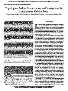
(a) Uncertainty in position before loop clo- (b) Uncertainty in position after sure. loop closure. Figure 1.4: Loop closure.

(Figure Courtesy of Paul Newman)

environment as well as the position of all the objects detected in the environment using cartesian coordinates in a global coordinate frame. As a result, objects’ positions and the geometric relations among them in an accurate map should be consistent with that of their real world geometry. Common examples of metrical maps are geographic maps (Figure 1.2a). Figure 1.2b shows a metrical map built by a robot using point cloud data from a laser range finder. A topological map on the other hand does not need to have a global coordinate frame and represents the environment as places/locations that are represented as nodes of a graph which can be connected by edges. Edges represent some sort of connectivity between the places. Adjacence is a common connectivity constraint in mobile robotic applications which means that two places should be connected if they are adjacent and vice versa. An important and advantageous property of topological maps is their independence of geometrical information about the environment. A traditional example of a topological map is a metro map (Figure 1.3a) which shows different stations as nodes and edges connecting pairs of nodes indicating traversability across them. Figure 1.3b illustrates an example topological map created in an indoor environment. Metric and topological mapping concepts will be discussed in detail in chapter 2.

5

Introduction

1.1.3

Loop Closure

Both metrical and topological approaches heavily rely on loop closure detection for successful map building. Loop closure is the process of asserting whether the robot is currently revisiting a previously location or is in a completely new location where the robot has never been before. Figure 1.4 depicts a situation where the robot revisits a location thereby forming a loop. The figure also shows uncertainty ellipses all along the robot’s trajectory whose size indicates the uncertainty in the robot’s position at the moment. If a loop closure is discovered at the time of the revisit, position uncertainty can be reduced and the necessary position correction can be propagated backwards throughout the trajectory. This is an example of loop closure in case of metrical map building and similar logic applies for topological mapping. In case of topological maps, loop closure captures the topological structure of the environment by creating edges between location nodes that are adjacent. However, loop closure is a challenging problem because of the following reasons: • Scalability: As the size of the map/environment increases, every new observation has to be compared with all the previous observations in the map. This is called the correspondence problem and is prominent in large-scale outdoor mapping and in particular topological mapping which is not even conscious of its metrical positioning. The problem intensifies depending on the observation dimensionality. For example, in case of observations represented as point clouds, a location signature dimensionality could be in the order of thousands and when using these signatures to solve the correspondence problem in a big map, the computational cost explodes. • Perceptual Aliasing: Different places in the environment look perceptually similar and may lead to false positives in correspondence evaluation. • Measurement Noise: Every sensor measurement is accompanied by a certain degree of noise. In addition to that, the environmental illumination which is quite variable plays an important role in complicating the correspondence problem. • Dynamic Objects: Dynamic objects are a problem in both indoor and outdoor environments and the correspondence evaluation should be robust to them. It is important to understand the difference between localization and loop closure. Loop closure has to classify each incoming observation as a revisited place or a completely new place. Where as, the localization problem holds a

6

Thesis Goals

presumption that the given observation definitely comes from some location in the given map and that location should be found. Hence loop closure is a much more complex problem than localization (GK99), (SAH04). Detailed literature on SLAM, mapping and loop closure can be found in chapter 2.

1.2

Thesis Goals

This thesis mainly addresses three problems each of which are discussed in the following subsections.

1.2.1

Loop closure for Topological Mapping

Problem Description: Vision based loop closure for topological map building in large scale outdoor environments using an inexpensive and uncalibrated omnidirectional camera. Many existing approaches (AFDM08), (ADMF09), (CN08), (CN09), (FEN07) to the topological mapping problem assume/construct dense topological maps. In a dense topological map every image acts as a place/node in the topological graph resulting in maps with as many nodes as the number of images in an acquisition sequence. While checking for a loop closure, the search space consists of all of these nodes and the computational complexity increases with the sequence size. Sparser topological maps can be built by partitioning an input image sequence and representing each partition as a node in the map. In the resulting map, each node represents a group of images rather than individual images. This kind of partitioning ensures that the images belonging to a node are sequentially contiguous and hence, spatially close, visually similar and collectively represent a place of the environment. In other words, a node represents a group of images belonging to a region or place in the environment, over which the visual similarity remains constant. Figure 1.5 illustrates a sparse/hierarchical topological map structure. This representation can be understood in two ways: 1. As a two-level hierarchical framework in which the first level represents the regions in the environment (as nodes) and the second level represents the images belonging to a particular region (images belonging to a node). 2. As a sparse topological map since the map is represented by nodes which are much fewer in number than the total number of images. Such a sparse/hierarchical mapping framework has several advantages.

7

Introduction

1111111111

34567 389ABCDBE6B4FB

2

2

2

2

2

2

1111111111 389ABCDBE6B4FB 9774B

BC 4C 5AF9C95

9FBC4C7BC 448B47

Figure 1.5: Sparse/Hierarchical topological map.

8

Thesis Goals

• Quick loop Closure: Facilitates a two step hierarchical loop closure. The first step is called the node level loop closure which retrieves the most similar nodes in the map. The second step called image level loop closure attempts to find the most similar image among the images belonging to the most similar nodes. The first step happens quickly (since the number of nodes will be lesser by many folds than the number of images) and boils down the search space from the whole map to a few nodes. Second phase of loop closure considers only a fraction of the total number of images and hence also happens fast. Consequently, the maps should be scalable to at least a few tens of thousands of images with the possibility of a realtime loop closure. • Accurate loop closure: To perform node level loop closure, all the images of the node are considered in evaluating its similarity to the query image. This process eliminates many unrelated places and perceptual aliasing situations from being considered in image level loop closure. Since the search space for image level loop closure becomes sparse, robust and computationally expensive matching techniques can be used for matching to further reduce false positives while retaining online operability. • Metric place representation: Instead of building a globally consistent metric map, one can represent the environment as a topologically connected set of places, each of which is metrically reconstructed from the sensor data. Since these maps have to be just metrically accurate, the computational complexity in mapping does not increase with the growth in number of observations unlike in global metrical mapping. • Place representation in maps can aid in accurate semantic labeling of topological map nodes (Ran10), (Ran12) that can be used for lifelong operation and navigation of robots. Places can also aid in providing stronger constraints for pose-graph SLAM (OLT06), (GSB09), (SP11) and topo-metric SLAM (LFP12). • Accurate and efficient map merging (EC12). However, the scope of this thesis is limited to the use of hierarchical representation for accurate and efficient loop closure and map building. Although a few of the existing topological mapping approaches use panoramic images from omnidirectional cameras or multi-camera rigs like LadyBug, they do take advantage of the rich 360 degree image representation. With a 360 degrees field of view, omnidirectional images do not suffer from objects going out of the field of view as the robot moves or rotates. As a result, even during robot translation, omnidirectional image appearance remains constant for a longer time as

9

Introduction

compared to the pinhole camera images. This property of omnidirectional images naturally supports the notion of places - regions of an environment over which the acquired images’ appearance remains similar. Another advantage of omnidirectional cameras is that one needs to traverse each path only once (irrespective of the direction of motion) in order to map the environment as opposed to the traditional cameras which demand at least two passes through a path each in two directions. However, inexpensive omnidirectional cameras generally produce image with poor resolution which can result in few feature matches on a given pair of images. Hence, the image similarity measures should be able to perform reliable matching even with a few feature matches.

1.2.2

Adaptive Visual Memory Update

Problem Description: Adaptive visual memory update mechanism for navigation in dynamic environments. Almost all the real world environments contain dynamic and semi-dynamic objects. For instance, consider an office environment, in which humans act as dynamic objects and furniture acts as semi-dynamic object(s) which are replaced or moved every once in a while. Visual memory of the robots should accommodate these changes and build a more consistent representation of the environment over time by giving higher weights to objects constantly observed at some places while reducing the weights and eventually discarding rarely observed or moving objects. Such constant update of visual memory should improve localization and navigation accuracy over time, while reducing the required computational resources for storage and computation of the visual memory.

1.2.3

A Multisensor Dataset Acquisition

Problem Description: Construction of a multi-sensor dataset for robotics and vision researchers. The need for publicly available datasets is always at its peak in robotics. Every dataset offers a unique challenge in testing a mobile robotic algorithm due to their difference in acquisition method, illumination conditions and environment type. Also, having multiple sensor data acquired simultaneously in the same environment makes it possible to test the effectiveness of a single sensor or a combination of multiple sensors in solving different problems. Acquiring a multi-sensor dataset poses an immense challenge due to the heavy data load incurred by the sensors and has to be handled carefully using multiple computers. Also the data acquired by various sensors connected across various computers needs to be properly synchronized in order to facilitate sensor fusion

10

Contributions

and several algorithms’ evaluation. Availability of complete and accurate groundtruth information is vital for evaluation of applications like loop closure, SLAM and visual odometry.

1.3

Contributions

• A sparse topological mapping framework is proposed which stores the map hierarchically. Novel hierarchical inverted files (HIF) are used to store the map and perform hierarchical loop closure efficiently. Traditional TFIDF similarity measure is combined with novel spatial and frequency heuristics for image similarity measurement. This framework is compared with two other state of the art techniques for sparse topological mapping in terms of efficiency, sparsity and accuracy. Modest loop closure recall rates without the use of any epi-polar geometry verification are achieved. • To improve the recall rates while maintaining the robustness of loop closure a second hierarchical mapping framework is proposed. VLAD features which have never been used in the robotics community have been used to model nodes. A spatial constraint specific to omnidirectional images is proposed for robustly matching and similarity evaluation of image pairs. The loop closure recall rates have been considerably improved while capping the computational complexity to allow real-time performance. The approach is compared to a contemporary approach: FABMAP 2.0 (CN10) in terms of the accuracy offered without even performing epi-polar geometry check. In another perspective, the approach yields better performance even on low-quality images with few feature matches. • The third contribution of this thesis is the formulation of a visual memory representation and update mechanisms for navigation in dynamic environments. Initial results on a small scale dataset supports the proposed mechanism. Very little research has been done on this problem and also evaluation of an approach becomes difficult due to a serious lack in common datasets. • The final contribution of this thesis is the detailed description of acquisition and construction of our multi-sensor dataset called the Institut Pascal Datasets (IPDS). The constructed dataset consists of 7 cameras, 2 laser range finders, odometry, IMU, a low-cost GPS and an RTK-GPS. A complete and precise ground truth has been provided throughout the sequence. This is the first dataset with an omnidirectional camera mounted on top of a car-like vehicle while traversing completely through an outdoor environment. The trajectories have been carefully planned to accommodate loops

11

Introduction

of varying lengths ranging from a few meters to a few hundreds of meters making the data suitable for evaluation of various mobile robotic and vision algorithms like SLAM, loop closure and visual odometry.

1.4

Structure

The present thesis is divided into 7 chapters. Chapter 2 discusses the related literature in detail while chapter 3 discusses the HIF based hierarchical mapping framework. An improved mapping framework using our novel spatial similarity measure for omnidirectional images and VLAD is discussed in chapter 4. A visual memory management for long term navigation approach and preliminary results are presented in chapter 5. Chapter 6 discusses the Institut Pascal DataSets (IPDS), our multi-sensor datasets, and finally chapter 7 contains my research conclusion and perspectives on future research.

1.5

Associated Publications

• Hemanth Korrapati, Youcef Mezouar, Appearance based Topological Mapping For Omnidirectional Cameras,Autonomous Robots. (Submitted, in review). • Hemanth Korrapati, Youcef Mezouar, Vision based Sparse Topological Mapping, Elsevier: Robotics ans Autonomous Systems. (Special Invitation, submitted) • Hemanth Korrapati, Ferit Uzer, Youcef Mezouar, Hierarchical Visual Mapping with Omnidirectional Images, IEEE/RSJ International Conference on Intelligent Robots and Systems (IROS), 2013, Tokya, Japan. • Hemanth Korrapati, Jonathan Courbon, Youcef Mezouar, Philippe Martinet, Image Sequence Partitioning for Outdoor Mapping, International Conference on Robotics and Automation (ICRA),2012, St.Paul, MN, USA. • Hemanth Korrapati, Jonathan Courbon, Youcef Mezouar, Topological Mapping with Image Sequence Partitioning, In 12th International Conference on Intelligent Autonomous System (IAS-12), Jeju Island, Korea, June 2012. Winner of the Best Oral Paper award. • Hemanth Korrapati, Youcef Mezouar, Philippe Martinet, Efficient Topological Mapping with Image Sequence Partitioning, European Conference on Mobile Robotics (ECMR), Orebro, Sweden, 2011.

12

Associated Publications

• H. Korrapati, J. Courbon, S. Alizon, F. Marmoiton, The Institut Pascal Data Sets : un jeu de données en extérieur, multicapteurs et datées avec réalité terrain, données d’étalonnage et outils logiciels, ORASIS 2013. • Hemanth Korrapati, Jonathan Courbon, Youcef Mezouar, Topological Mapping with Image Sequence Partitioning, Book Chapter in Frontiers of Intelligent Autonomous Systems, Springer series: Studies in Computational Intelligence,Vol. 466 • J. Courbon, H. Korrapati, Y. Mezouar, Adaptive Visual Memory For Mobile Robot Navigation In Dynamic Environment, In IEEE Intelligent Vehicles Symposium (IV’12), Alcalá de Henares, Spain, June 2012. • J. Courbon, H. Korrapati, Y. Mezouar, Visual Memory Update For LifeLong Robot Navigation, In 12th International Conference on Intelligent Autonomous System (IAS-12), Jeju Island, Korea, June 2012.

13

Introduction

14

2 Literature Review This chapter provides the necessary literature review in the lines of the work presented in this thesis. A brief review of mobile robotic SLAM will be provided followed by a detailed review of appearance based topological mapping. Subsequently, hybrid mapping approaches and visual memory based navigation approaches are reviewed.

2.1

SLAM

Mobile robotic SLAM aims at building a map of an environment while at the same time localizing itself in the map. The robot’s trajectory and the location of landmarks (objects in the environment) are estimated online without any a priori information about them. Figure 2.1 provides an idea of how the robot’s trajectory and landmark locations are linked from each others’ perspective. Deducing a solution to the SLAM problem is a notable achievement of the robotics community. Although theoretically SLAM is a solved problem, there remain many problems in practical implementation of generic SLAM systems in real world. A statistical basis to SLAM was provided in (SC86) and (DW88) which describes how landmarks are geometrically inter-related and a way to evaluate their uncertainty. This work concludes the necessity of high degree of correlation among the landmark location estimates which improve with successive observations. In the landmark paper (SSC90), it has been pointed out that the relative observations acquired during a mobile robot motion are all correlated with each other due to the common error in the robot’s position estimate. Hence, it has been suggested that a consistent solution for simultaneous localization and mapping would need a joint estimate of the robot’s state and the landmark states all of which need to be updated on each observation of a new landmark. Apart from

15

Literature Review

Figure 2.1: SLAM problem: Landmarks being observed at different positions along the robot’s trajectory. Figure courtesy: Time Bailey (DWB06)

not considering the convergence properties of the map, the computational complexity increases in the order of the number of landmarks squared. With the advent of the paper (HDWN96), it has been realized that the SLAM problem was convergent and the solution grew better with the landmark correlations. An ameliorated theory on convergence along with initial results were provided in (Cso97). Kalman Filter representation of the SLAM problem of (HK99) and probabilistic formulation of localization and mapping problems of (TBF98) were brought together for the first time in 1999 laying foundations for a kalman filter based probabilistic SLAM. EKF-SLAM (Extended Kalman Filter SLAM) is one of the popular variants of SLAM whose basis was laid in (SSC90) and later combined with probabilistic recursive bayesian framework. The probabilistic framework uses a two step recursive prediction and update process. The basic version of EKF-SLAM has several disadvantages, including its fragility to incorrect correspondences arising from loop closure false positives. Also EKF-SLAM demands that the landmark locations and the joint covariance be updated with every observation which can become a computational bottleneck. However, efficient variants of EKF-SLAM with many thousands of landmarks were demonstrated (LF00), (GN01). Recent approaches with sub-mapping strategies (PTN08), (BNLT04) were able to further reduce the computational complexity of EKF-SLAM solutions. EKF-SLAM linearizes the actual non-linear motion and observation models which can induce

16

SLAM

significant errors into the system. Variants using Unscented Kalman Filters and Iterated Extended Kalman Filters partly address this issue. Finally, the most important isue is the assumption that all the covariances can be approximated as gaussians leading to multi-modal density distributions. Although some success has been achieved with EKF-SLAM, it still does not scale to maps with millions of landmarks. Consequently, a particle filter based SLAM popularly known as FastSLAM has been introduced in (MTKW02) based on previously proposed approaches (Mur99), (TBF00). FastSLAM works by recursive Monte Carlo sampling by nonlinearly modelling the process and with a non-gaussian model for pose distribution, two of the major disadvantages of EKFSLAM. However, it still linearizes the observation model and is normally considered as a reasonable approximation. Due to the high-dimensional nature of the SLAM problem application of particle filters directly is infeasible and hence the state space is partitioned using Rao-Blackwellization (R-B). As a result, the joint state can be represented using the product of vehicle component and conditional map component, and the probability distribution is on the robot’s trajectory rather than a single pose. Conditioning on the trajectory makes the landmarks independent and makes it possible for the map to be represented by a set of independent gaussians, making the computational complexity linear rather than a quadratic complexity as in case of EKF-SLAM. FastSLAM 2.0 (MTRW03), differs from the original method (MTKW02) in the proposal distributions for particle filtering and is more efficient. The re-sampling step during filter updates in FastSLAM causes loss of memory of the trajectory history and hence only applicable to scenarios which are in accordance with exponentially forgetting their past. This results in failure of FastSLAM based approaches to produce a consistent map over long and loopy trajectories. The scalability issue of SLAM has been further tackled using canonical parametrization of SLAM distribution. The Extended Information Filter (EIF) (May79) approach uses this canonical form to describe gaussians by inverse matrix (inverse covariance) and an information vector as opposed to a dense covariance matrix and a mean vector as in traditional approaches. EIF works analogous to EKF in a two step update and predict fashion. EIF greatly speeds up the update step but slows down the predict step (complexity quadratic in the number of landmarks) and moreover it requires an O(n3 ) matrix inversion operation to extract mean from the information matrix. Totally, EIF is only as good as EKF and not any better. Although EIF is not a good approach, the idea of canonical representation caught the attention of some researchers (TLK+ 04), (FH01). It has been realized that in feature based SLAM majority of the off-diagonal elements of the information matrix are near-zero values. (TLK+ 04) nullifies these values giving rise to a Sparse Extended Information Filter (SEIF), an extension to EIF which significantly speeds up the predict step giving rise to a near-constant time solution to

17

Literature Review

SLAM. Based on the idea of (SK86) which represents canocical parametrization using gaussian markov random fields in which small values of the information matrix correspond to weak links. (Pas03) and (Fre06) break these weak links and approximate the graphical model as a sparse tree structure and use Thin Junction Tree Filter and Treemap filter respectively. SLAM has been solved in a batch processing framework as well. Maximum Likelihood Estimation (MLE) has been used in (TBF05), (DMS00), (FC04), (FLD05) to optimize a full non-linear log-likelihood function over the entire history of robot positions and observations. The algorithm is iterative and robust to data association and linearization errors. GraphSLAM (TBF05) is another batch algorithm which represents robot positions and observations as nodes and measurement constraints as edges. GraphSLAM work iteratively and at each iteration, the linearization yields a sparse information matrix on which a variable elimination algorithm is applied. Much more details about various types of SLAM can be found in (TBF05), (DWB06) and (BDW06).

2.2

Appearance Based Topological Mapping

As introduced in the previous chapter, topological maps are represented as graphs with nodes representing places and edges representing some form of connectivity across the corresponding nodes/places. In fact, what nodes and edges represent in a topological map depends on the application, the sensor type and the algorithms used to build them. Unlike metrical maps, topological maps do not need a global frame of reference and hence are completely independent of metrical information about the environment. Despite being quite common, there is no accurate consensus about what topological maps are and how they should be constructed. The major assumption underlying the topological approach to mapping is that there is a level of abstraction of the underlying environment at which actions are deterministic (RK04). Cognitive mapping theories which try to explain the human understanding of large scale space suggest that cognitive maps have strong topological nature (Yea88), (CKK95), (Kui00), (Lyn60), (PI67), (HM71). Several non probabilistic theories (CN01), (KB91), (RK04) and probabilistic approaches (RMD06), (RD06a) have been proposed for topological mapping all of which are limited to maps with few landmarks (in the order of a hundred or two). Vision or image based topological mapping approaches are commonly referred as Appearance Based Topological Mapping (ABTM) and is the main theme of this thesis. ABTM is becoming more popular because of the following reasons: • Images provide rich information in the form of colors and textures from the environment.

18


• Compact data representation as images as opposed to huge point clouds provided by range sensors like laser range finders or LIDARS. Range sensors are the other major class of sensors used in mobile robotic applications. • Semantic environment understanding is relatively easier with visual data than with range data. • Cheaply available. However, possibility of extracting range information from images is limited and computationally expensive with the exception of stereo images which can provide accurate depth information only up to a short range. Some mapping applications which need depth/range information have successfully used range sensors in conjunction with vision by calibrating them together enabling them to project each one’s readings on to the other’s.

2.2.1

Loop Closure vs Content Based Image Retrieval

Loop closure which was discussed in chapter 1 is an integral part of topological mapping. In fact, pure topological mapping completely relies on loop closure detection for accurate map generation as loop closure decides when to add edges in the topological graph. In the context of appearance based topological mapping, given a query image, the loop closure module searches if the image belongs to a previously visited place (therefore the image of that place). If it belongs to a previously visited place, then the current image and the previous image are linked in the topological graph. Loop closure is also commonly known as place recognition. Wrong loop closures (false positives and false negatives) influence the accuracy of the maps. False positives create spurious edges between nodes and can lead to undesirable results when using the topological map for navigation. False negatives on the other hand are not as dangerous but can result in a graph with redundant nodes. Hence a loop closure approach should aim at producing zero false positives and minimizing number of false negatives. The loop closure problem holds similarities with the Content Based Image Retrieval (CBIR) approaches in the computer vision community with some exceptions. CBIR typically aims at image search, retrieving the most similar images from a large database or index given a query. A query can be anything ranging from textual keywords of the image description (in case of web image search), textures, colors, an object in the image or even a complete image. Image based loop closure resembles CBIR when the query is an image. CBIR and loop closure differ in the following ways: • CBIR aims to retrieve the most relevant images in the decreasing order of relevance. Loop closure expects an accurate image match and a null result

19

Literature Review

if no match occurs. Hence it is important to distinguish a matching case from a no-match case. • In CBIR each image in the database is independent of all others while in a mapping approach images are stored in the order of acquisition and hence while performing loop closure, availability of neighboring images of any given reference image of the database is guaranteed. Availability of neighboring images can be used to impose additional temporal constraints (BHK12), (BF11) on matching and hence reduces the chance of false matches. • while CBIR is only image based, loop closure can take advantage of information from other sensors ranging from the robot’s proprioceptive sensors like odometers to external sensors like laser range finders or radars. However, there is a lot that is adapted from CBIR research pertaining to global/local feature extraction and efficient registration/indexing of images. A brief review of some recent CBIR techniques for quantization and matching relevant to appearance based loop closure application is provided in sections 2.2.3.1.

2.2.2

Loop Closure with Global Image Features

The aim of global image features is to describe an image using a single signature which can be thought of as a vector of numerical values. Global features are represented as vectors and serve as compact image signatures for image registration and retrieval purposes. Several global image features have been proposed over the past two decades and have been successfully used in localization and loop closure applications. Global color histograms computed over RGB and HSV color spaces of panoramic images are used for localization in topological maps (UN00). Localization is performed by nearest neighbor learning and achieved an accuracy between 87% and 98% in both indoor and outdoor datasets. An eigen-image representation has been used in (JL99) for localization in a set of panoramic images. Zero Phase Representation (ZPR) (Paj99) has been used to bring the panoramic images into a rotation invariant format. ZPR Images are projected into a low-dimensional eigen space to facilitate efficient localization. An auto-correlation technique to produce rotation invariant images which are projected into eigen-spaces for localization in (AIYT98). Similarly, (KVBM01) adopts a PCA based dimensionality reduction in a probabilistic framework for localization in a set of images. Fourier coefficients of panoramic images are used as their signatures for localization in topological maps in (MMI04). It has been shown that these signa-

20


tures which are simple to compute are sufficient for achieving good localization accuracy. All the above discussed global image descriptors are not robust to illumination variation, occlusion and large view-point changes. Another popular global image descriptor (OT01), (OT+ 06) is GIST which aims to produce a low dimensional representation of an image. A set of perceptual dimensions namely naturalness, openness, roughness, expansion and ruggedness that represent the dominant spatial structure of a scene are estimates using spectral and coarsely localized information. Therefore the input image is segmented into a 4 × 4 grid over which orientation histograms are extracted and represented in a single vector. GIST has been successfully used in image search and retrieval (LWZ+ 08), image completion (HE07) and web scale image search (TFW08). (LZ12) projects GIST descriptors into a low dimensional space and uses particle filter to detect loop closures. A modified version of GIST called omni-GIST has been proposed in (MCKG10) for topological mapping which will be discussed in chapter 3. However, GIST is known for its lack of discriminative power and have been proven to perform badly in comparison with local image features in a bag-of-words representation (DJS+ 09). (TS05) proposes a topological mapping algorithm which represents places as fingerprints constructed from omnidirectional images and laser range scans. Color patches and edges from omnidirectional images and corners extracted from laser scans are used to construct the fingerprint signatures. These fingerprints of periodically acquired sensor readings are grouped based on the self-similarity of the environment to form nodes of the topological map. Another descriptor similarly extracted from dominant vertical lines in unwrapped panoramas is introduced in (LSP+ 09). Each detected vertical line is described using its color information in YUV color space and augmented to the global image descriptor called DP-FACT. These descriptors are used for automatic node addition in topological maps and loop closure. Gobor-GIST feature descriptors are used in (LZ12) for representing images compactly to be used in loop closure. This approach has been used on popular datasets to obtain good recall rates.

2.2.3

Local Image Features

Local image features are patterns in an image which differ from their immediate neighborhood. The difference could be in one or more appearance metrics like color, texture, intensity, etc. Unlike global features, local features are robust to occlusions, variances in illumination and viewing angle, rotation and scale (up to a certain degree). Different types of local features are available in literature: • Corner based: Harris corner detector (HS88), Harris-Laplace detector (MS04),

21

Literature Review

Harris-Affine detector (Lin95), (LG97), SUSAN (Smallest Univalue Segment Assimilating Nucleus) (SB97), FAST (Features from Accelerated Segment Test) (RD06b). • Blob based: Hessian detector, Hessian-Laplace/Affine, SIFT (Scale Invariant Feature Transform) (Low04b), SURF (Speeded Up Robust Features) (BTG08). • Region based: IBR (Intensity Based Regions) (TVG00), (TVG04), MSER (Maximally Stable Extensible Regions) (MLS05). Which feature to use depends on the desired application. For example, Harris corners and SUSAN are invariant to rotation and translation of images ; HarrisLaplace and Hessian-Laplace are invariant to scale changes while Harris-Affine, Hessian-Affine and MSER are invariant to affine transformations; SIFT is invariant to uniform scaling, orientation, and partially invariant to affine distortion and illumination changes ; SURF is invariant to rotation/non-rotation and scale, and possesses high repeatability and distinctive characteristics. Much more details about all the feature detectors can be found in (TM08). Each detected feature can be described using a descriptor extracted over the region centered around the feature location (also called keypoint). The most common types of descriptors are SIFT, SURF, ORB (Orientation BRIEF) (RRKB11), BRISK (LCS11) and BRIEF (CLO+ 12). FAST features/corners being described by recently introduced binary descriptors ORB, BRIEF, BRISK are getting popular due to their quick computation. Also, binary descriptors facilitate efficient feature matching and quantization based on Hamming distance. Apart from the computational advantage, binary descriptors are not as robust as regular descriptors like SIFT or SURF. In our applications SURF detectors and descriptors are used as they provide a good trade-off between robustness and computational time and are known to produce better results in some cases (VL10). Despite their robustness, local features are not as compact as global descriptors. There can be hundreds or even thousands of local feature detected on each image and for applications like image search this could become a real computational bottleneck. For example, lets consider an image with 500 SIFT features each of 128 dimensions which has to be matched against another image with an equal number of features; a brute force approach will take at least 500 ×500 ×128 operations while a nearest neighbor approach can be relatively efficient but memory intensive; if one has to repeat the same process for a large database of images in an image search application, computational time per search operation will be huge and increases linearly with the number of images. In order to tackle this problem, feature quantization and efficient matching schemes have been proposed which will be the focus of next subsection.

22


2.2.3.1

Feature Quantization & Matching

Feature Quantization is the process which quantizes each local feature descriptor into visual words. In other words, each multi-dimensional feature descriptor is to be represented by (quantized to) a single integer value (visual word). (SZ03) is one of the first works in computer vision community that presents a notable feature quantization approach motivated from text retrieval approaches like TFIDF (Term Frequency Inverse Document Frequency) and inverted files. To adapt the text retrieval approaches, images also must be represented by words. This is done by quantizing feature descriptors into visual words using a bagof-words visual vocabulary model which was motivated from (Sch01), (LM01). A bag of words vocabulary is learned on training images by applying k-means clustering on the feature descriptors extracted from them. The number of clusters k formed by k-means clustering represents the size of the vocabulary (number of possible visual word assignments). Given a feature descriptor to be quantized, its quantized value (visual word) is the index of the closest cluster of the k clusters in the bag of words model. The closeness of a cluster is determined by the euclidean distance between the given descriptor and the cluster’s centroid. A visual word histogram which indicates how many instances of each visual word are present in a particular image, is built for every image to facilitate matching. Figure 2.2 illustrates a toy example of a bag of words training and representation. The bag of words model used in (SZ03) is flat and requires a computational complexity linear in the vocabulary size to quantize (to find the closest cluster). As a result, it is not computationally feasible for very large vocabularies. To make this bag of words model scalable, (NS06) proposed a tree representation for the vocabulary called vocabulary tree. A vocabulary tree is constructed by applying hierarchical k-means clustering on the training data. Vocabulary size represented by a vocabulary tree depends on its branching factor (k) and the number of levels (l). Figure 2.3 demonstrates a toy example of a vocabulary tree. The vocabulary size is given by the number of leaf nodes of the tree (k l ). To quantize a given descriptor, its euclidean distance to all the k cluster centroids of the root node is computed. The closest centroid is selected and the distances to all of its k children to the query vector are evaluated. This process is repeated l times such that the query descriptor reaches a leaf node; the descriptor is said to be quantized and is assigned a quantized value corresponding to the leaf node to which it is quantized. Computational cost of the quantization operation is logarithmic in the number of leaf nodes. Hence, even if the vocabulary size is increased, the quantization cost will be increased just by a log factor, making them suitable for large vocabularies. An approximative k-means algorithm combined with a randomized forest of kd-trees was used for quantization of descriptors in (PCI+ 07). An improvement

23

Literature Review

(a) Feature extraction from train- (b) Visual vocabulary construcing images. tion by feature clustering.

(c) Feature quantization using vi- (d) Visual word histogram of the sual vocabulary on a query image. query image. Figure 2.2: A hypothetical bag of words model construction and feature quantization. Figure 2.2a: Training images on which two dimensional feature descriptors are extracted. Figure 2.2b: K-means clustering of the feature descriptor space where k = 4. Figure 2.2c: Feature descriptors extracted on the query image, quantized to their respective clusters and those cluster ids are treated as the visual words of the corresponding descriptors. Figure 2.2d: Using the extracted visual words a histogram representation of the query image is built which can be used for image matching. (Figure courtesy of Kristen Grauman’s lecture notes.)

24


(a) Feature Space

(b) Hierarchical Clustering

(c) Vocabulary Tree

(d) Quantization

Figure 2.3: A toy example of vocabulary tree building. Figure 2.3a: A two dimensional feature descriptor space. Figure 2.3b: Hierarchical clustering of the feature space with two levels(l = 2) and a branching factor(k = 3). Top level clusters are represented by green circles and separated by green lines and similarly, the second level by blue. Figure 2.3c: A vocabulary tree representation of the hierarchical clusters. Figure 2.3d: Given query image patches, the leaf nodes to which the query patches are quantized is shown. (Figure courtesy of David Nister (NS06).)

25

Literature Review

using soft quantization which improved quantization accuracy was proposed by the same authors in (PCI+ 08b). Hamming-embedding technique was proposed in (JDS08a) to be used on top of the bag of words quantization over small vocabularies to improve the discriminative power of descriptors. All of (SZ03), (PCI+ 07), (PCI+ 08b), (JDS08a) use a geometric verification step in order to validate the hypotheses obtained after bag of words ranking of images. (SZ03) uses epi-polar geometry, (PCI+ 07) uses the shape information from affine invariant interest points and (JDS08a) embeds weak geometric consistency directly into the ranking step. However, all these approaches increase the memory for indexing the images. (PCM09) uses a memory efficient way to store the shape information of interest region for geometric verification. Inverted files were used in all of the above discussed approaches for efficiently indexing the quantized visual words of images. They were first used to index documents for efficient retrieval and are the most common data structures for document retrieval tasks in search engines (ZMR98). As the name suggests, inverted files are the inverted representations of a document: A single document can be thought of a list of words while an inverted file of a word is a list of references to the documents in which that word occurred. Every word in the vocabulary has an associated inverted file. The strength of inverted files comes from its ability to answer the question: In which documents did a particular word occur and how many times ? This is a basic version of inverted files and much more complicated models exist, with the central aim being the same as above. Starting from (SZ03), many researchers from computer vision (NS06), (JDS08b), (JDS08a), (PCM09), (PCI+ 07), (PCI+ 08b) and robotics (AFDM08), (ADMF09), (FEN07) began using inverted files for image retrieval tasks. The only differences needed to accommodate were to use images instead of documents and visual words in place of textual words. An example of inverted file usage with images is illustrated in Figure 2.4.

2.2.4

Loop Closure with Local Image Features

A variety of appearance based localization techniques that use local features have been introduced over the past decade (SD98), (DJ00), (WBB05) (LK06), (WCZ05), (Fil07), (FSD06), (SBS07), (MSG+ 07), (MGS07). Extrema of the density of edge distribution of images are used as landmarks for localization in (SD98), (DJ00). Features invariant to limited scale variation and translation are used for in (WBB05) in a monte carlo localization scheme. In (LK06), a localization framework based on a reduced set of local salient features is used. Bag of words framework has been used in (WCZ05) and in (Fil07) to localize a robot in a set of images. A Bernouilli mixture model has been used to learn conditional dependences between visual words in (FSD06). A city scale location recognition

26


123456 17859A5B CDE56

Figure 2.4: Inverted file representation for images. The first and second columns of a row of an inverted file contain the index of image in which the word occurred previously and the corresponding occurrence frequency respectively.

has been proposed in (SBS07) that supports the idea of a wider branching factor in vocabulary tree and uses a reduced set of informative features for place representation and localization. A radial line descriptor is introduced in (MSG+ 07) to perform hierarchical localization in omnidirectional images. Radial line descriptors are extracted based on the color, intensity and geometry information, which are then used in a pyramidal matching framework to perform localization. Appearance based loop closure problem as discussed earlier is much more challenging than localization and has been gaining popularity over the last decade. A loop closure technique relying on (NS06) is proposed in (FEN07) as a part of a topological mapping, localization and navigation system. (BZK09) reduces the size of the topological maps by using connected dominating sets, thereby keeping only the most important images. SIFT features were used for image matching in these two approaches. Most of the loop closure approaches discussed so far just operate on a precomputed set of image features or visual words. A path breaking work reported in (Fil07) introduced an incremental localization and mapping framework. This work proposed a framework in which visual words extracted from images are incrementally added to the map and therefore can be immediately available for localization tasks. (AFDM08) extends this framework by introducing a recursive bayesian filter framework that combines the image similarity information temporally over a sequence of images. Loop closure posterior is obtained by filtering and normalizing the loop closure likelihoods. The loop closure candidates with a high posterior are geometrically verified using epi-polar geometry. Another important constribution of this work is to perform reverse scoring using inverted files. The ingenuity of reverse scoring is that it limits the complexity of image

27

Literature Review

similarity evaluation to be in the order of number of visual words of the query image as opposed to other approaches whose complexity increases with the number of images in the map. However the disadvantage of reverse scoring is that it cannot accomodate negative observations into similarity scoring. (ADMF09) extends (AFDM08) by using odometry in conjunction with visual data to form a topological map with metric information embedded over the edges. A probabilistic loop closure technique called FABMAP that uses a generative model over visual words is proposed in (CN08), (CN09), (CN10). Visual words are obtained by quantizing features using kd-trees. Pairwise relations between visual words are learned using a Chow-Liu tree (CL68). In (CN08) Chow-Liu tree constructs a graph such that the maximum co-occurrence probability can be extracted. These co-occurrence probabilities are used in evaluating image to image similarities which are combined using a recursive bayesian filter. Candidates with posterior higher than a threshold are considered for geometrical verification step. FABMAP is extended in (CN09), (CN10) by adapting an inverted file framework to improve performance. The authors call this technique FABMAP 2.0 which is evaluated on two large outdoor datasets of 70 km and 1000 km demonstrating the accuracy and computational gains provided by the approach. A hierarchical loop closure approach is proposed in (CGLR+ 10). The first phase of loop closure involves a fast similarity computation using a bag of words framework. The images that achieved the highest degree of similarity are then given to the Conditional Random Field (CRF) algorithm which is computationally more demanding. (MGLLC11) discusses a loop closure algorithm that weights visual words based on their potential to generate right or wrong loop closures. Loop closure accuracy is determined based on the depth map generated from the stereo cameras. Visual words supporting true loop closures get their importance weight improved while the visual words leading to wrong loop closures get their weight diminished. A time efficient loop closure approach is proposed in (GLT11) which gains much of its efficiency by using BRIEF (CLO+ 12) feature descriptors. As mentioned earlier, BRIEF descriptors are binary codes and are very fast to compute and are helpful in efficient matching and quantization approaches. Most of the popular loop closure techniques like (AFDM08), (ADMF09), (CN08), (CN09), (CN10), (GLT11), (FEN07) use epi-polar geometry verification step to validate the loop closure result. An algorithm which uses a similarity measure based on dynamic programming to match images using appearance and relative positions of local features, is proposed in (AD09). The probability of loop closures is computed using a Markov Random Field (MRF). BRIEF-Gist descriptors of an image which are computed using the local BRIEF descriptors are used in (SP11) for loop closure detection. The loop closure algorithm is used as a front-end for a pose-graph SLAM.

28


A separate class of algorithms based on the analysis of similarity matrices have been proposed in the past. These algorithms compute the similarity between each reading and every other reading and represent the similarities in the form of a similarity matrix. (SAH04) uses a technique that uses SIFT features for similarity evaluation and a similarity matrix analysis. A graph cut algorithm is applied on the similarity matrix to extract clusters of similar images in (ZBK05). The perceptual aliasing problem has been addressed in (HN05b), (HN05a), (HN05c), (NCH06), (HN07) by applying Singular Value Decomposition (SVD) on the similarity matrix to eliminate the effects of self-similarity in the environment. All the above discussed approaches consider each acquired image as a node/place in the topological map. Many of these techniques do not even consider the mapping problem but just solve the loop closure problem. These techniques can be understood as dense topological mapping since there will be as many nodes in the map as the number of observations. There are several techniques to represent the map using fewer nodes by partitioning the input image sequence such that all the images with similar appearance are represented by a single node in the topological graph. Since the number of nodes in this process will be fewer than the total number of input images, the resulting maps are called sparse topological maps. The remainder of this section reviews the sparse mapping approaches from the literature. In (ZBK07), (ZBK05) topological maps are built for indoor environments. They segment the topological graph of the environment using normalized graphcuts algorithm resulting in subgraphs corresponding to convex areas in the environment. In (KLY05) SIFT features were used to perform matching over a sequence of images. They detect transitions between individual indoor locations depending on the number of SIFT features which can be successfully matched between the successive frames. In (TS05) fingerprint of an acquired image is generated using omni-directional image and laser readings, and these fingerprints are used in loop closure. If the similarity is above a threshold the image is added to the existing node and if not a new node is formed. Change point detection has been used for indoor place segmentation in (Ran10). All the above works experimented on indoor environments which contain convex spaces (like rooms) and are relatively easier to be partitioned when compared to outdoor environments which in general do not have clear boundaries that separate places. An incremental spectral clustering technique is applied for topological mapping in (VDL07). The images are clustered using the similarities in the similarity matrix which are then represented as nodes of the topological map. Nodes are constructed using incremental spectral clustering over the affinity matrix of the images, producing a sparse topological graph. Another ISP technique was presented in (NVP10) which used mean optical flow vector length to signal changes in scene and nodes are formed only at those locations. (MCKG10) performs sparse

29

Literature Review

mapping through ISP using rotation invariant GIST (OT01) features called omnigist. An ISP technique is presented in (CRF12) which adapts the GIST descriptor to spherical representation of omnidirectional images. However this approach was just evaluated in terms of its power of image sequence segmentation but not used in any mapping or loop closure application. The present thesis deals with the construction of the above discussed sparse topological maps.

2.3

Hybrid Mapping Approaches

Metrical maps which are computationally expensive are rich in information about the environment while topological maps on the other hand are scalable to large environment but cannot provide any metrical information about the environment. Both metrical and topological maps are powerful in their own way of representation. Hence, a map that can provide both metrical and topological information while being scalable to large environments is always desirable. Such maps are called Hybrid maps. As in the case of topological maps, there is no single definition of how a hybrid map should be represented. However, the following two types of Hybrid maps are common: • The map is topologically represented as a graph of places with the edges encoding metrical relations between the nodes. That is, the translation and rotation required to reach from one node to another node is encoded in the edges. These maps are generally built by optimising the topological graphs whose edges encode odometry or other position estimates, using the loop closures as constraints. The class of algorithms which produce these maps are called pose-graph SLAM algorithms (LM97), (OLT06), (FS06), (DK06), (GSB09), (KGS+ 11), (KJR+ 11), (KRD08), (KGK+ 10), (SP12). The loop closure module which produces constraints is called the front-end and the optimizer is called the back-end. The pose-graph SLAM approaches are motivated by GraphSLAM techniques discussed earlier. • The map is represented by nodes which store accurate local metric information and these nodes are topologically connected to give rise to a global map. These approaches are commonly called hierarchical maps or sub-mapping approaches (BNLT04, ENT05, KA04, KMB+ 04, MBK04, TB96, BFMG08, LFP12). Our loop closure approach can serve as the front-end for Hybrid map building using a pose-graph SLAM framework.

30

Visual Memory for Long-Term Operations

2.4

Visual Memory for Long-Term Operations

What is a visual memory ? Is it not a map ? We can say that visual memory is a subtype of maps that is used just for robot localization and navigation to perform their daily tasks. However, the name visual memory is inspired from its biological similarity with human visual memory used for navigation. Human visual memory can be defined as: Visual memory occurs over a broad time range spanning from eye moments to years in order to visually navigate to a previously visited location. A visual memory should be able to adapt to the changes in a dynamic environment where the appearance of places changes constantly because of the movement of different objects to different places. Humans, with their highly developed cognitive abilities, discriminate between dynamic and static objects and represent their visual memory accordingly. The same should be achieved by robots to accurately localize and perform navigation in dynamic environments for long term. In the field of visual navigation in dynamic environments, a large part of the literature deals with transient changes. The robot’s environment is generally split in a static part and an ephemeral (potentially moving) objects. Two solutions can be used to deal with this situation. The first solution consists of identifying the elements which are not consistent with a static model of the environment. This is usually bypassed with geometric consistency of view matching. The second solution consists of tracking moving objects as proposed in the context of VSLAM in (BR07), (WM09). These objects can then be integrated to the map building process as in (BR07) or rejected as in (WM09). However, these solutions may improve the current localization but cannot handle long-term changes in the structure of the environment. Very little work has been devoted to accommodate long lasting changes into the visual memory. In feature-based visual SLAM approaches, features accumulate over time (which can be seen as a map update) but obsolete features are not discarded. As a result, the required memory and processing power grow continuously with time. In (HS09), the evaluation of the quality of the localization allows to rank landmarks and to eliminate less useful ones. In (ATD07), the initial map is supposed to be partially correct and a robust method for global place recognition in scenes subject to changes over long periods of time is proposed. As the reference view is never modified, this approach may be inefficient after some time. It seems more promising to modify the reference views as proposed in (DD08) ,(BSBC10) ,(DCD11). The information model used in those works is based on the human memory model proposed in (AS68) and the concepts of short-term and long-term memories. Basically, reference views are stored in a Long Term Memory (LTM). When features have been seen in many views during the localization step, they are transfered from the Short Term Memory (STM) to the long-term

31

Literature Review

memory (if they are not already in it) and missing features are forgotten (which are deleted after some time). The updates of the memories are based on a finite state machine in (DD08), (DCD11) and on Feature Stability Histograms built using a voting scheme in (BSBC10). It is reported that localization performance is improved with respect to a static map. However, these works only deal with topological maps. In (DCD11), the strategy proposed in (DD08) is improved by adding metrical data enabling the estimation of the robot’s heading for navigation. To this end, 3D spheres containing the observed visual features have been incorporated in the map for each node.

2.5

Conclusion

The previous sections briefly discussed the related literature in SLAM, appearance based topological mapping and long-term visual memory maintenance for navigation. A major part of our work falls in the lines of sparse topological map construction (discussed in section 2.2.4) with loop closure as the core of the algorithm. We propose two techniques for topological mapping: The first one is based on Hierarchical Inverted Files (HIF) (a derivative of inverted files discussed in 2.2.3.1) along with novel heuristic constraints for loop closure. The second one uses global VLAD descriptors in conjunction with a spatial constraint on visual words to perform loop closure. Both these approaches are evaluated on the grounds of recall rates obtained without performing an epi-polar geometry verification like other techniques discussed in section 2.2.4. Instead we use a relative motion model to validate the loop closure candidate hypotheses. Our approach is compared with a two recent sparse mapping approaches and a recent loop closure approach called FABMAP 2.0. The second part of our work deals with visual memory for navigation. Unlike existing approaches discussed in section 2.4, our approach caters a generic visual memory update framework for topological and metrical maps that can be updated over time. As in (DCD11), our goal is the improvement of the full navigation process, which includes localization and path following stages. Experimental evaluation in indoor datasets has been reported.

32

3 Loop Closure Using Hierarchical Inverted Files This chapter discusses a hierarchical loop closure framework for building sparse topological maps as discussed in section 1.2.1. Sparse maps are built by partitioning the incoming image sequence and representing each partition as a node of the topological map. Each parition contains images of a place or region of the environment over which the visual similarity is consistent. Breaking a sequence of images acquired by the robot into nodes/places is called Image Sequence Partitioning (ISP) and we achieve this using a local feature matching based similarity evaluation. To facilitate hierarchical map representation and feature indexing, a data structure called Hierarchical Inverted File (HIF) is proposed. As opposed to the traditional inverted files (ZdMNBY00), (NS06), HIFs store features hierarchically in two levels - node level and image level. HIFs enable loop closure at two resolutions - a coarse node level loop closure which finds the most similar node and a finer image level loop closure which pin-points the most similar image inside a node. Constraints that exploit spatial locations and occurrence frequency of features in images are used to strengthen the image level loop closure and thereby eliminate false positives. A filter taking advantage of the temporal consistency of loop closure which also depends upon the vehicle velocity is used in validating loop closures. Experimentation was performed using omni-directional images from two of our own outdoor datasets and panoramic images from the popular NewCollege dataset (SBC+ 09), all of which are publicly available. We compare our approach to two other mapping approaches that use ISP: the first is based on GIST (TMFR03), (MCKG10) and the second one uses Optical Flow (NVP10). Sparsity and accuracy of maps constructed using different ISP techniques are evaluated and the

33

Loop Closure Using Hierarchical Inverted Files

Figure 3.1: A global modular view of our topological mapping framework.

power of HIF representation in time efficient loop closure is demonstrated.

3.1

Framework Overview

Figure 3.1 depicts a global overview of our framework. Given a query image (a newly acquired image), local image features are extracted and quantized into visual words. Any of the rich variety of existing local feature detectors like SIFT, SURF, etc.. can be used as local image features. Quantization of local image features into visual words is performed using a vocabulary tree (section 2.2.3.1) learned on a training dataset. The features extracted from the query image are then used for a node level loop closure check. Basically, node level loop closure evaluates the similarity of the query image to all the reference nodes (can also be called node-image similarity) of the topological map. On occurrence of a node level loop closure, which means that the query image is probably acquired at a previously visited place(s)/node(s) in the map, the member images of those nodes are tabbed as reference images for a more thorough image level loop closure.

34

Image Sequence Partitioning

Image level loop closure involves an image-to-image similarity evaluation of the query image with respect to all the reference images, and filtering the similarity for valid loop closures. Howbeit, if an image level loop closure does not occur (if the query image is not similar to any reference image), the image is considered for comparison with the current place node. Likewise, if a node level loop closure does not occur, then too the query image is considered for comparison with the current place. As can be seen in the figure, similarity evaluation of the query image to the current place node mainly constitutes Image Sequence Partionting (ISP). At this point, it is decided whether the query image belongs to the current place and if it is too dissimilar to the current place, a new place/node is created with the query image augmented to it. We call the first image added to a node as the primordial image and it is features of this image which are used for ISP. The following sections discuss each of the above discussed modules in detail.

3.2


Image sequence Partitioning (ISP) answers the question: Does the query image belong to the current place or to a new place ? We use a Local Feature Matching (LFM) based similarity criterion to measure similarity between the current place and the query image. Let It be the query image, Nc be the current place node and Ip be the primordial image of the current place. A query image It is considered similar to the current node Nc if the percentage of matches between the of query image feature set Ft and the primordial image feature set Fp is above a threshold Tisp . It ∈ Nc ⇐⇒ M(Fp , Ft ) ≥ Tisp (3.1) Where M(Fp , Ft ) is the function computing the percentage of matches between the two feature descriptor sets: X φ(fit , Fp ) M(Fp , Ft ) =

fit ∈Ft

min(n(Fp ), n(Ft ))

.100

(3.2)

Where φ(fip , Ft ) is an indicator function signaling a match given by, ( N N (f t ,Fp ) 1 if N N 21 (fit ,Fp ) ≤ α t p i φ(fi , F ) = 0 otherwise Where NN 1 (fiq , Fr ) is the distance of the first nearest neighbor of the feature in the set of feature descriptors of Fr . Similarly, NN 2 (fiq , Fr ) is the distance of the second nearest neighbor. This heuristic is called the nearest neighbor ratio

fiq

35


(NN-ratio) test first proposed in (Low04a). The intuition behind this matching heuristic is that if the first nearest neighbor is from the same object as the query feature descriptor and the second nearest neighbor is from a different object, then the first and second nearest neighbors should be separated by a significant distance. From the above equation, the second nearest neighbor distance should be more than or equal to (1 − α) ∗ 100 percent of the nearest neighbor distance. Essentially, the second nearest neighbor determines if the nearest neighbor is a valid one or not. For example, in our algorithms we use a value of α = 0.8, which means that the second nearest neighbor should be at least 20% more than that of nearest neighbor for a match. This process can lead to a few false positives in general. However, in the present scenario, the representative image and the query images are acquired at spatially close locations and this fact projects a much slimmer chance of false positives. LFM based partitioning makes sure that all the images in a node are at least Tisp percent similar to the primordial image and the similarity of every other pair of images of a node is definitely more than Tisp percent.

3.3

Visual Word Indexing

Visual words which are the quantized values of local image features, simplify and accelerate feature matching tasks due to their compact representation. In our framework, visual words are used for node and image level loop closure operations. Storing visual words in the memory in such a way that facilitates their easy access is called indexing and can result in an optimized loop closure performance. Indexing is an essential need for numerous text retrieval applications and is commonly performed using a data structure called invertedf ile (ZMR98). As discussed in section 2.2.3.1, the strength of inverted files comes from its ability to answer the question: In which documents did a particular word occur and how many times ? Starting from (SZ03), many researchers from computer vision (NS06), (JDS08b) and robotics (AFDM08), (ADMF09), (FEN07) began using inverted files for image retrieval tasks. The only differences needed to accommodate were to use images instead of documents and visual words (obtained by quantizing local image features) in place of textual words. Several recent approaches have utilized inverted file based similarity evaluation (AFDM08), (ADMF09), (CN10) for loop closure problems. However, inverted files propose a flat representation and therefore cannot be directly applied to our approach because of the hierarchical structure of our maps. We need to modify the inverted file structure to suit our hierarchical map representation as well as loop closure at different resolution (node and image level). Hence, a derivative of inverted file representation which we call Hierarchical Inverted File (HIF) is used

36

Visual Word Indexing

Figure 3.2: Hierarchical Inverted Files illustrating the node level and image level information hierarchies.

for indexing image and node memberships of visual words in our framework.

3.3.1

Hierarchical Inverted Files

To exploit the hierarchical structure of our topological maps we propose Hierarchical Inverted Files (HIF). HIFs organize the visual word information in two levels of hierarchy - at node and image levels. Such a representation gives rise to flexibility in probing node and image membership information of visual words. Given a visual word wi , HIFs answer the following two questions, vital for an efficient loop closure: • In which nodes did a particular visual word wi occur ? • In which images of a particular node Nj did a particular visual word occur ? HIFs answer both these queries with the membership information as well as the occurrence frequency statistics. Figure 3.2 illustrates an example of HIF representation. The first level of a HIF stores node level information, i.e. the nodes in which a visual word wi occurred previously. At the second, attached to each node is the list of images belonging to that node in which the visual word wi occurred. Taking one more step forward, a HIF can be modified to accommodate keypoint locations of the visual words. Instead of just storing the occurrence frequency of

37


Figure 3.3: Hierarchical Inverted File with spatial information embedded.

visual words, a list of keypoints of the visual words in the corresponding image can be stored. We refer to these HIFs as Spatial HIFs (Figure 3.3). A Spatial HIF can answer an additional query apart from the two queries answered by a HIF: what are the keypoint locations of a particular visual word in an image belonging to a particular node?. Such a flexible representation proves useful in evaluating spatial similarities of images efficiently while performing loop closure, as we shall see in the later sections. Through the remainder of this chapter wherever a HIF is mentioned it inherently means a Spatial HIF.

3.4

Loop Closure

As we have already seen in Figure 3.1 loop closure is performed in two stages: first at node level and then at image level. The current section details these two loop closure processes in detail.

3.4.1

Node Level Loop Closure

Node level loop closure (NLLC) aims to find the most similar nodes to the query image Iq . In other words, the nodes or places that have a high likelihood to have generated the query image, should be found. However, node level loop closure might even produce an empty set of similar nodes which means that the image is not similar and hence not generated from any of the nodes in the map indicating a no loop closure event. A no loop closure event means that the image belongs to either the current place or a new place, which we decide by performing an ISP.

38

Loop Closure

To perform an NLLC the set of all nodes in the map NR are considered. ∀i,

Ni ∈ NR

Algorithm 1 details the steps involved in node level loop closure. The query image is input to the algorithm. Visual words extracted from it are used in computing node similarities using the node level information of the words’ HIFs. Regular TF-IDF (Term Frequency-Inverse Document Frequency) (SM86) scoring is used to compute all the node-image similarities (line 7). A regular TF-IDF weight of a visual word wi is evaluated as, n(NR ) n(wi , Nj ) (3.3) × log T f Idf (wi, Nj ) = n(w, Nj ) n(wi , NR ) The first term in equation 3.3 is called the term frequency (TF) and the second term is called inverse document frequency (IDF). TFIDF is a popular scoring technique used in document retrieval (SM86). TF measures the importance of a word in a document and increases with the number of occurrences of the word in the document. This is the most common variant of TF among a few others. Whereas IDF measures the importance of a word across the whole document collection by assigning high scores to rare words (which are seen only in a few documents) than the words commonly occurring in many documents. The purpose of IDF is to assign high weights to discriminative words. In our context, TF is the ratio of occurrence frequency of a visual word wi in the node Nj to the total number of visual words in the Nj . IDF is the logarithm of ratio of total number of nodes in the set NR to the number of nodes of NR containing visual word wi . The vector of node similarities SN , is then normalized with respect to the highest score and all the normalized scores (except the current node) above a threshold θN will be treated as most similar nodes N∗ . ∀i, ∀i,

Ni ∈ N∗

SN [i] =

SN [i] SN max

if SN [i] ≥ θN

and Ni 6= Nc

(3.4) (3.5)

SNmax is the maximum similarity value in SN . However, SNmax is always the similarity of the current place node, since the query image is recent and hence largely similar to the current place than any other. Post normalization, all the scores will be in the range [0, 1] and hence the parameter θN should belong to this range. The intuition behind this type of normalization is that if the robot is actually revisiting a place then node corresponding to the previous visit will have a similarity value comparable to that of the current place. In the event

39


of no loop closure, N∗ will be empty and hence ISP is performed. This way of normalization-to-highest is effective in eliminating wrong matches due to noise and helps in detecting no loop closure events. Normalization-to-highest is also a simple alternative to using average image (AFDM08), (ADMF09) and mean field approximation (CN08), (CN09), (CN10). Node level loop closure makes use of only the node level information of the HIFs which is just a fraction of the total data and hence happens quicker than when a flat inverted file is used. Moreover the number of nodes in N∗ will be few and hence their member images form a tiny fraction of the total number of images in the map. As a result, the search space for image level loop closure is greatly reduced. Algorithm 1 Node Level Loop Closure using HIF 1: procedure Node_Level_Loop_Closure(It ) 2: 3: 4: 5: 6: 7: 8: 9: 10: 11: 12: 13:

SN =Array(size_of(NR )) Wt =extract_and_quantize_Features(It ) for each word wit in Wt do HIF i =get_hierarchical_inverted_file(wit ) for each node Nj in HIF i do SN [j] = SN [j] + T f Idf (wit , Nj ) end for end for s=normalize_to_highest_element(s) N∗ =get_most_similar_nodes(s) return N∗ end procedure

3.4.2

Image Level Loop Closure

Image level loop closure intends to signal a loop closure event by finding most similar images from the reference image set IR , as well as a no loop closure event in case of no similar images. The reference image set IR is a union of all member images of the nodes in N∗ . [ INi IR = Ni ∈N∗

Where INi is the set of member images of node Ni . Similarity computation of these reference images to query image (image-to-image similarity) is detailed in Algorithm 2. For each visual word of the query image its corresponding HIF

40

Loop Closure

is probed for the images corresponding to the nodes of N∗ . Similarity scores of the corresponding scores are updated using a product of STF-IDF weight, a spatial similarity weight and a frequency constraint weight (line 9). Each of these weighting schemes are discussed subsequently. Algorithm 2 Image Level Loop Closure Algorithm 1: procedure Image_Level_Loop_Closure(N∗ , It ) 2: 3: 4: 5: 6: 7: 8: 9: 10: 11: 12: 13: 14: 15: 16: 17:

SI =Array(M ) ⊲ M - Total number of images in the map. t W =get_visual_words(It ) for each word wit in W do HIF i =get_hierarchical_inverted_file(wit ) for each node Nj in N∗ do N IF i j =get_inverted_file_of_node(HIF i , Nj ) n for each entry Ik in IF i j do SI [k] = SI [k] + (ST f Idf (wi , Ik ) × ss(wi , Kt , Kr ) × f c(wi , It , Ik )) end for end for end for smooth_and_normalize(SI ) I∗ =get_winner_from_histogram(H) I∗ =validate_loop_closures(I∗ ) return I∗ end procedure

3.4.2.1

STF-IDF

The STF-IDF is another variant of the regular TF-IDF scoring in which STF stands for Sub-linearly scaled Term Frequency. STF-IDF differs from TF-IDF in the term frequency factor which is non-linearly scaled by a log function instead of a normalized linear scaling of the traditional definition. TF assigns high weights to features which occur many times in an image, which is counter-intuitive in case of image matching. For example, lets consider a reference image containing a lot of occurrences of a visual word wi . While considering this image for loop closure, its TF becomes very high due to the importance of wi in that image, thereby producing high similarity contribution towards images containing even a single occurrence of the visual word. STF on the other hand just scales the occurrence

41


frequency instead of normalizing it. ST F − IDF (wi , Ik ) = (1 + log(n(wi , Ik ))).log 3.4.2.2

n(I) n(wi , I)

(3.6)

Spatial Similarity

The Spatial similarity measure uses keypoint locations of visual words in the query and reference image (obtained from HIFs) in measuring their spatial consistency. The fact that robot motion is locally planar enforces the objects of an image acquired at a certain place to occupy the same vertical space (y-coordinates) when the robot exactly revisits a place. This constraint is used to assign higher similarities to matched visual words whose y-coordinates of keypoints are close. The closer they are, the higher their corresponding spatial similarity. However, this becomes a problem when there are unequal number of same visual words in the query and reference images. Finding the exact correspondences between the multiple features complicates this problem but in practice we found that the following heuristic works well. Consider a visual word wi and let K1 and K2 be the sets of keypoints locations of wi in two images. Without loss of generality, let n(K1 ) ≤ n(K2 ), where n(.) is the number of keypoints operation. Our heuristic is applied as follows: 1. For a keypoint ki1 in K1 , find the closest keypoint kj2 in K2 in terms of y-coordinates. kj2 ∈ K2 : j = arg min|ki1 .y − kp2 .y| p

2. The distance |ki1 .y − kj2 .y| is added to a list D. 3. ki1 and kj2 are discarded and the iteration is repeated from step 1 until K1 is completely empty. Finally, a list of distances D are obtained which are used to compute the spatial similarity measure using an exponential kernel. Y ss(wi , Kq , Kr ) = g(D[j]; 0, σsp), j

−(x − µ)2 2σsp 2

where g(x; µ, σ) = exp 

 = exp  

−

X

(D[j])

j

σsp 2

42

2

   

!

(3.7)

Loop Closure

Where σsp is the kernel width parameter which determines the score variation with the variation of y-coordinate distances. Spatial similarity constraint ensures higher weights to visual word matches which are close in vertical space and lower weights to dispersed visual word matches. 3.4.2.3

Frequency Constraint

The frequency constraint enforces the two images to have the similar counts of each visual word if they are acquired in the same place. If Iq and Ir are the query and reference images, then the frequency constraint also given by an exponential kernel is, ! f c(wi , Iq , Ir ) = exp

n((wi , Iq ) − n(wi , Ik ))2 σf 2

(3.8)

Where σf is the kernel width parameter which controls how strongly the visual word frequency difference can influence the similarity score. Frequency constraint compensates for the information loss incurred due to the unaccountability of inverted file based similarity evaluation which ignores the difference in occurrence frequency of the matched visual words in two images. 3.4.2.4

Smoothing & Normalization

Once the image similarity vector (SI ) computation using algorithm 2 is complete, the vector of similarities need to be smoothed and normalized. Due to the noises accumulated over several processes ranging from image acquisition to feature extraction, detection and quantization, image similarities might be slightly dispersed across their neighbors and hence smoothing is essential. Smoothing is achieved by convolving the similarities vector SI with a gaussian window W (equation (3.9) and (3.10)). SI = SI ∗ W (µ, σsm )

(3.9)

W (µ, σsm ) = [g(−2; 0, σsm ),g(−1; 0, σsm), g(0; 0, σsm), g(1; 0, σsm), g(2; 0, σsm)]

(3.10)

The vector SI is then normalized with respect to the highest similarity in the same way as the node similarity vector SN in equation (3.4), and the images with similarities above a threshold θI are retained. Although a minor difference in this case is that we ignore all the recently acquired δ (a small number) images.

43


Figure 3.4: Figure showing a re-traversal. Green trajectory is the previous traversal and the red trajectory is the current traversal.

The justification lies in the fact that temporal proximity of images implies spatial proximity which in turn gives high similarities to those images always.

∀i, ∀i, 3.4.2.5

SI [i] SImax ∗ Ii ∈ I if SI [i] ≥ θI SI [i] =

(3.11) and Ii 6= Ic ,

c ∈ [c − δ, c]

Loop Closure Validation

After the above mentioned operations, the vector SI contains similarity values of few images which are likely to be loop closures. There remains two tasks before obtaining the final loop closures: first task of extracting hypotheses and the second of validating the hypotheses. All the clusters of contiguous non-zero similarities in SI , are detected. In each cluster, the highest similarity value is retained while the other similarities are nullified, thereby leaving only the highest similarity value (corresponding image) as a loop closure hypothesis. To validate a loop closure, we rely on its temporal consistency: A loop closure spans several time steps and hence contains several match pairs. Figure 3.4 shows an example of a re-traversal (loop closure) which occurs over a period of time and several image match pairs supporting loop closure. The image match pairs are called loop closure candidates. Loop closure candidates are different from loop closure hypothesis in that the latter is just a hypothesis and should be validated before becoming a candidate. To summarize, a valid loop closure consists of a set

44

Loop Closure

of loop closure candidates which are obtained by validating potential loop closure hypotheses. Now the question remains: how to add a loop closure hypothesis to the set of loop closure candidates ? Let Ir and It′ be the latest reference and query image match pair that is the most recent candidate of a loop closure L, and let It be the current query image. It can pair up with a reference image Ir′ to form a loop closure hypothesis that can be added to L only if it satisfies the following conditions. (It , Ip ) ∈ L only if

t − t′ ≤ s and |r − r ′ | ∈ [⌈a(1 − ∆)⌉, ⌈a(1 + ∆)⌉]

(3.12)

Where s is the skip parameter which decides how many loop closure candidates of the previous images can go unidentified before encountering another loop closure candidate. a is the interval parameter that estimates the interval which should contain the loop closure candidate reference images. a is estimated using the velocity difference between the previous traversal and the current traversal and ∆ error parameter that defines the percentage of error in calculation. t−1 X d (I , I ) i i+1 ′ ≥1 a = arg min i=t (3.13) n X n d (Ij , Ij+1) j=r

d (Ii , Ii+1 ) is the distance traveled by the robot between the acquisition of images Ii and Ii+1 which can be obtained from the robot’s odometry. The ratio of sum of distances of the previous images and the reference images estimates how many reference images to skip starting from Ir . However, in case of constant velocity (previous traversal and current traversal with same velocity) which is the case in many of the available datasets including ours, a can be estimated much more simply. In such case, t′ will be equal to n and hence a = t − t′ . Finally, a loop closure and all its candidates is valid only if it contains at least p loop closure candidates. In our implementation, we use s = 3, p = 3, ∆ = 0.30 along with a constant velocity assumption. Even though odometry data drifts over long trajectories, it is locally accurate across small time steps. As opposed to other loop closures approaches which use motion model (BHK12), (BF11), our model compares the previous traversal speed with the re-traversal speed in estimating the next loop closure location. Hence we call the presented model, relative motion model. Every valid loop closure candidate is used in map update by adding the candidate’s query image to the node corresponding to the reference image.

45


8768EB4

8768EB4

123456278

8768EB4

8768EB4

56278492ABCBCDEF

Figure 3.5: Image partitioning and canonicalizing for omni-gist features extraction.

3.5

Similar Approaches

This section provides a brief introduction to two recent approaches based on GIST and optical flow respectively, which also aim to build topological maps by partitioning image sequences and simultaneously use the maps to perform loop closure. Comparisons with respect to map sparsity, accuracy and computational time are provided in the section 3.6.

3.5.1

GIST

GIST is a global image feature introduced by (OT01), (TMFR03) as a part of a context-based vision system for object and place recognition. GIST produces a feature vector corresponding to the average response to steerable filters employed at different scales and orientations computed over 4 x 4 sub-windows. The advantages of GIST are fast descriptor computation and compact representation of the spatial structure of images using a single global signature vector. The topological mapping approach using GIST has been adopted from (MCKG10) which uses a modified version of GIST called omni-gist specifically meant for omni-directional images. Each omni-directional image is split into four parts and GIST feature descriptors are extracted on each of the four parts. Figure 3.5 visually depicts the omni-directional image splitting and canonical representation as four segments. These four descriptors act as sub-descriptors which when put together form an omni-gist descriptor G = {G1 , G2 , G3 , G4 }. To facilitate efficient distance computation between among omni-gist descriptors, each sub-descriptor of is quantized and represented by a single visual word giving rise to a four word quantized omni-gist descriptor g = {g1 , g2, g3 , g4 }. The quantized is performed using a bag of words framework. Given two quantized omni-gist descriptors g and g′ , the distance/similarity between them is given by the average of the minimum

46

Similar Approaches

cyclic distance between the two descriptors as in equation (3.14). 1 ′ ′ ′ ′ (min (|g1234 − g1234 |, |g1234 − g2341 |, |g1234 − g3412 |, |g1234 − g4123 |)) 4 (3.14) The notation g2341 indicates that the gist visual words are organized in the order 2, 3, 4 and 1 for the euclidean distance operation |.|. The |.| operation is the sum of euclidean distances between the cluster centroids to which the visual words belong. Nodes and Representative Features: Each node represents a sequence of images belonging to a place and is represented by the centroid of the member image omni-gist descriptors. Similarity to Current Place: Given a query image its, similarity with the representative feature of current place is evaluated, which if within certain threshold g Tlow , the image is added to the current place node. Addition of an image to a node involves updating the representative feature (centroid) taking the new feature into account. If the image does not satisfy the threshold, it is considered for image level loop closure. Loop Closure: Distances between the new omni-gist feature and all node representative features is computed and the top 30% of the closest nodes are g selected. Of these, nodes closer than a threshold Thigh and having a number of g local SURF feature matches above certain threshold Tsurf are considered as loop closures and the appropriate nodes are updated. However, when there is no loop closure, then a new node is created and the query image augmented to it. g g Parameters Tlow and Thigh are the lower and higher threshold values which control the evaluation of similarity to current place and a different place in the map respectively. The intuition is that, for the current image to be added to the current place the similarity between the two should be very high and hence the threshold is low. While if the image belongs to another place other than the current one, the similarity would not be too close and hence a higher value of threshold is used. The original approach also contains sub-clusters in each node, which we omitted in the above discussion for brevity and clarity, but not in the implementation. dist(g, g′ ) =

3.5.2

Optical Flow

Optical flow based key place detection algorithm of (NVP10) is the second approach which aims at the same outcomes as our approach. The basis of this algorithm is the fact that change in scene (change in place) triggers significant change in optical flow magnitude. The places where a significant optical flow occurs are called key locations of the environment.

47


8

Mean Optical Flow Vector Length

7

6

5

4

3

2

1

0 0

1000

2000

3000

Image Id

4000

5000

6000

7000

Figure 3.6: Change points in mean optical flow vector length. Red stars indicate peaks and green stars indicate valleys in optical flow. Both of them signal key locations.

Optical flow is computed on image corners detected using Canny edge detector. Lucas-Kanade tracking algorithm is used for tracking the corners across frames. Only stable features (those that are present over several consecutive frames) are considered for optical flow evaluation. Optical flow vectors are to be normalized by subtracting vehicle velocity from the obtained optical flow values and by balancing the rotations performed by the robot. However, in our experiments, the robot travels with constant velocity and undergoes in-plane rotation. Hence, we eliminate the optical flow normalization step. The flow vectors are converted into polar coordinates and the mean optical flow vector length is computed, which when exceeds a certain threshold Tof triggers a key location possibility. Figure 3.6 shows a graph of mean optical flow vector length with triggered key locations at peaks and valleys. Nodes and Representative Features: Nodes are formed whenever key locations (scene change) are triggered by the change in mean optical flow value. Representative features of a node are the SIFT features of the image which triggers scene change. The new node formed due to every scene change is added to the map. Loop Closure: Loop closure is performed on every trigger of a scene change using quantized SIFT features (using a visual vocabulary). The top three nodes in terms of SIFT feature matches are retrieved of which the images with more than 50% matches are considered loop closures. In case of a successful loop closure, the nodes are joined by an edge in the topological graph.

48

Experiments

3.5.3

Differences

The two discussed topological mapping approaches differ from our approach in several ways. The most important difference is that given a query image, our approach attempts to check if it associates to a previously visited place and then considers adding to current node or creating new node. GIST based technique tries to assign each new image to the current place and then attempts loop closure and the same goes with optical flow technique. This model may ignore some loop closures as there is no guarantee that a place change is triggered at exactly same point in the environment every time, giving rise to false negatives. The second difference is that we use the same features (USURF-64) for comparison with current place, node level loop closure and image level loop closure. While the other two methods detect two kinds of features for camparison with current place and loop closure respectively, which causes additional computational load. In fact, the computational load might be a significant motivation behind their choice of not considering loop closure as a priority over addition to current place, given a query image.

3.6 3.6.1

Experiments Datasets and Platform

Three image sequences in total are used in evaluating our approach. Out of the three sequences, two are our own publicly available datasets1 and the third one is the NewCollege dataset2 . A VIPALAB platform is used for acquisition of our datasets, which is a carlike vehicle designed to serve as a prototype for research and development in autonomous urban transport vehicles. The platform has an on-board computer, an odometry system and an IMU (Inertial Measurement Unit), and can be manually driven using a control panel inside the vehicle or autonomously using the on-board computer. The system also contains several other sensors of which we are only interested in a omni-directional camera (provides gray-level images) and an RTK-GPS. The omni-directional camera is mounted on top of the vehicle to be at a height of 2 meters from the ground and the RTK-GPS is mounted such that it coincides with the rear-axle of the vehicle. RTK-GPS data (10 hz) is accurate upto 5cm accuracy and serves as ground-truth for loop closure validation. 1

Dataset acquisition supported by our laboratory: http://hemanthk.me/joomla/index.php/ipdataset 2 http://www.robots.ox.ac.uk/NewCollegeData/

49

Institut Pascal.

Hosted at


Sequence PAVIN (IP) Cezeaux (IP) NewCollege

#(Images) 8002 80913 7854

Traj. 1.3 km 15.4 km 2.2 km

Vel. 2.3 m/sec 2.5 m/sec 1.0 m/sec

FPS 15 hz 15 hz 3 hz

(a) Datasets Description

Sequence PAVIN (IP) Cezeaux (IP) NewCollege

FPS 2 hz 2 hz 1.5 hz

#(Images) 1144 11571 3977

(b) Data used for Experimentation. Table 3.1: Datasets Description. (Traj.=Trajectory Length, Vel.=Average Acquisition Velocity, FPS=Images Frames acquired Per Second)

Our two sequences PAVIN and CEZEAUX are named so after the places where they were acquired. PAVIN is an artificial village which simulates urban and rural environments with tarred roads, rural-style roads, road markers, traffic signals, roundabouts and junctions. CEZEAUX is the area surrounding Institut Pascal and the Blaise Pascal University and is a semi-urban style environment with roads, buildings, lawns and vegetation on either sides of the road. Much more details about VIPALAB and various other sequences can be found in chapter 6. Due to the low quality of omni-directional images, these sequences especially the CEZEAUX sequence offers a tough challenge for loop closure. From the NewCollege dataset, panoramic images acquired with a LadyBug camera are used. Due to the lack of completely accurate GPS data on NewCollege dataset, ground-truth tagging was performed by manual inspection. The datasets contain huge number of images (refer to Table 3.1a), however, much smaller subsets are used in our experiments. More precisely, only around two images per second are considered, resulting 3977 images for NewCollege sequence, 1144 for PAVIN sequence and 11571 for Cezeaux sequence (refer to Table 3.1b). Loop closure accuracies are measured by precision/recall values. Precision is the ratio of number of true loop closures detected (true positives) to the total number of loop closures detected (true positives and false positives). Recall is the ratio of true loop closures detected to the total number of existing true loop closures (sum of true positives and false negatives). In other words, precision measures how accurate the retrieved loop closures are and recall measures what

50

Experiments

Parameter Name Variable Match Percentage for ISP Tisp NN-ratio threshold α Node Similarity cut-off θN Spatial Similarity kernel width σsp Frequency Constraint kernel width σf Smoothing kernel width σsm Image Similarity cut-off θI

Value 40 0.8 0.5 6 2/3 2 0.7

(a) LFM+HIF based mapping parameters.

Parameter Name GIST Current place similarity threshold GIST loop closure similarity threshold No. of SURF matches Mean Optical Flow Threshold

Var. g Tlow g Thigh g Tsurf Tof

Val. 0.08 0.2 30 0.03

(b) GIST and Optical Flow based mapping parameters Table 3.2: Parameters. (Var.=Variable, Val.=Value)

percentage of the total loop closures are retrieved. A loop closure is considered true positive if the query and reference images are acquired at less than 5 meters distance according to ground truth. All our algorithms runs on a laptop computer equipped with an intel core i7 under linux.

3.6.2

Parameters

This subsection discusses various parameters used for loop closure detection which were introduced in the previous sections. Table 3.2a lists all the parameters used for loop closure detection using our Local Feature Based (LFM) based approach. The nearest neighbor ratio parameter value of α = 0.8 is observed to attain a good accuracy in feature matching while producing higher number of matches. Rest of the parameters and the values assigned to them are described in the subsequent sections related to sparsity and accuracy of the loop closure. The parameters for the GIST and optical flow based mapping approaches are listed in Table 3.2b and their assignment will be justified in the next subsections. As local image features, USURF-64 (the 64-dimensional upright variant of SURF) have been used. Two separate vocabularies are learned as vocabulary

51


(a) Raw omni-directional image.

(b) Masked omni-directional image for Optical Flow.

(c) Unwrapped omni-directional image. Figure 3.7: Raw, masked and unwrapped variants of an omni-directional image.

trees with branching factor (k = 6) and levels (l = 6), the first one for PAVIN and CEZEAUX sequences and the second one for NewCollege dataset. The PAVIN+CEZEAUX vocabulary is learned on the features extracted from 20% of randomly selected images from each of PAVIN and CEZEAUX sequences. Similarly, the NewCollege vocabulary is learned on 20% of randomly selected images from NewCollege datset. In LFM approach, omni-directional images are unwrapped using (Pro) and represented as a panoramic image (Figure 3.7c) before feature extraction is performed. For GIST based approach, omni-directional images are directly used. However, for optical flow (OF) based approach, the frontal and backward portions of the images are masked out as shown in Figure 3.7b. This step is necessary to eliminate features which appear in the robot’s direction of motion in the image which despite not generating any optical flow contribute in reducing the mean optical flow vector length.

3.6.3

Sparsity and Accuracy

Sparsity is the number of nodes required to represent a topological map. The fewer the number of nodes, higher the sparsity. However, higher sparsity does not imply map accuracy. In fact, maps can even be represented by as few as 10

52

Experiments

nodes irrespective of the number of images used to build them, provided the ISP threshold is sufficiently relaxed. In overly sparse maps, representative features of a node represent huge number of images and hence become more general rather than thoroughly representing a particular place of the environment. As a result, missing out true loop closure candidates during node level loop closure (NLLC) is likely. Due to such weak node level loop closure (NLLC) many true loop closure candidate images may not even be considered for image level loop closure leading to a loss in recall. Hence a good sparsity for a map is that which produces 100% recall rate in NLLC. Conjointly, a good precision means that only necessary loop closure candidate nodes are selected and hence image level loop closure can be sped up. In LFM+HIF approach, the parameter Tisp controls the node size and hence the map sparsity. Sparsity of the map along with the node similarity cut-off threshold θN plays a key role in NLLC accuracy. Achieving 100% recall in NLLC is important to atleast have a possibility of performing image level loop closure with full recall. The percentage of matches (Tisp ) is varied and the resulting map size along with the highest precision/recall values are illustrated in Table 3.3a for two different values of θN . We can see that Tisp = 40 and θN = 0.5 achieve the most sparse maps and highest NLLC precision (56% on PAVIN, 48% on CEZEAUX and 53% on NewCollege) with full recall. Tables 3.3b and 3.3c show the sparsity and loop closure precision using GIST and OF based approaches. These two approaches are tested only on the PAVIN and CEZEAUX datasets leaving out the NewCollege dataset due to lack of omnidirectional images for GIST and the lack of orientation information for masking frontal and backward views of panoramic images for optical flow based mapping. As mentioned before performing optical flow on a full omni-directional or panoramic image causes very small and erroneous mean optical flow vector lengths. For GIST based mapping, it has been observed that the threshold g Tlow = 0.08 which controls the current scene augmentation is ideal and any deviation affected the loop closure accuracy to a large extent. However, variance of g Thigh which controls loop closure produces much different results and its value of 0.2 produces best loop closure precision in both datasets. In OF based approach, the parameter Tof = 0.03 produces the best sparsity as well as recall rate. Among the two approaches, GIST appraoch acheives higher recall (42% on PAVIN and 11% on CEZEAUX) than that of OF (26% on PAVIN and 6% on CEZEAUX). It should also be noted that in GIST and optical flow approaches, node and image level loop closures are not separate and hence the recall values presented in Tables 3.3b and 3.3c are the total loop closure recalls. To summarize, the most sparse maps on PAVIN are produced by GIST followed by OF and LFM+HIF techniques. On CEZEAUX, OF wins in terms of sparsity over GIST and LFM+HIF. Although LFM+HIF looses to GIST and OF

53


1

1 stfidf−spat−freq stfidf−spat stfidf−freq stfidf tfidf

0.9 0.95

Precision

Precision

0.8

0.9 stfidf−spat−freq stfidf−spat stfidf−freq stfidf tfidf

0.85

0.7

0.6

0.5 0.4

0.8 0.3 0.75 0.55

0.6

0.65

0.7

0.75

Recall

0.8

0.85

0.9

0.2 0.1

0.95

0.2

0.3

(a) PAVIN

0.4

0.5

Recall

0.6

0.7

0.8

(b) CEZEAUX

100

Precision

95

90

stfidf−spat−freq stfidf−spat stfidf−freq stfidf tfidf

85

80

75 55

60

65

70

75

Recall

80

85

90

95

(c) NewCollege Figure 3.8: Precision-Recall graphs on various sequences. Figures 3.8a, 3.8b, 3.8c show loop closure precision-recall graphs obtained on different variants of the proposed LFM+HIF based approach.

in terms of sparsity, it has its advantages in terms of ILLC accuracy as we shall see in the later discussions. Image level loop closure accuracies on the three sequences using five different variants of the image similarity computation in LFM+HIF mapping are shown in Figures 3.8a,3.8b, 3.8c as precision-recall graphs. The graphs are generated by varying image similarity cut-off θI , spatial similarity kernel width σsp , and frequency constraint kernel width σf . For example, the stfidf-spat-freq variant is the one proposed in the previous section for image level loop closure in which, stfidf indicates STF-IDF weighting, "spat" indicates spatial constraint, and "freq" indicates frequency constraint weightings. Similarly accuracies obtained using four other variants with and without certain weightings (and named appropriately)

54

Experiments

PAVIN

Tisp

Nds.

CEZEAUX

Prec. Prec. Nds. (θN = (θN = 0.4) 0.5)

NewCollege

Prec. Prec. Nds. (θN = (θN = 0.4) 0.5)

Prec. Prec. (θN = (θN = 0.4) 0.5)

30%

90

-

-

665

-

-

280

-

-

40%

169

53%

56%

1663

42%

48%

360

45%

53%

50%

310

31%

44%

2645

28%

29%

517

36%

39%

60%

492

22%

36%

4590

19%

24%

834

21%

27%

70%

614

20%

24%

9002

8%

13%

1123

10%

15%

(a) Sparsity varying with Tisp (LFM+HIF mapping) and NLLC precision with 100% recall on the corresponding map with θN = 0.4 and θN = 0.5. g Thigh

PAVIN

CEZEAUX

Tof

Nds. Prec. Nds. Prec. 0.1

955

0.2

375

0.3

125

0.4

38

7245

42%

2341 11%

25% -

CEZEAUX

Nds. Prec. Nds. Prec.

3%

36%

PAVIN

0.01

1023

0.02

432

987

-

0.03

133

342

-

0.04

96

g (b) Sparsity varying with Thigh (GIST based mapping) and loop closure recall (with 100% precision) on the obtained maps.

-%

19% 26% 3%

8627 4532

-% -%

874

6%

497

-

(c) Sparsity varying with Tof (Optical flow based mapping) and loop closure recall (with 100% precision) on the obtained maps.

Table 3.3: Sparsity varying with ISP thresholds and loop closure precision on the corresponding maps. (Nds. = No.of Nodes, Prec. = Precision). Empty cells indicate that 100% precision is not possible for any recall value for that particular parameter configuration.

55


0.9

0.8 tfidf−reg

tfidf−reg 0.8

0.7

0.7 0.6

Precision

Precision

0.6 0.5 0.4

0.5

0.4

0.3 0.3 0.2 0.2

0.1 0 0.72

0.74

0.76

0.78

0.8

0.82

0.84

Recall

0.86

0.88

0.1 0.24

0.9

0.26

(a) PAVIN

0.28

0.3

0.32

0.34

Recall

0.36

0.38

0.4

0.42

(b) CEZEAUX

95 tfidf−reg 90

Precision

85

80

75

70

65

60 72

74

76

78

80

82

Recall

84

86

88

90

92

(c) NewCollege Figure 3.9: Figures 3.9a, 3.9b, 3.9c show precision-recall graphs obtained on the regular TFIDF based approach (no ISP) without geometric verification.

56

Experiments

are plotted alongside. Figures 3.9a, 3.9b, 3.9c show loop closure precision-recall graphs on the same sequences using just TF-IDF and a bayesian filter (as proposed in (AFDM08) ) without using ISP or HIF. However, the final RANSAC based epi-polar geometry verification step was not performed to obtain these results to enable fairness in comparison with our approach which does not use epi-polar geometric verification for loop closure validation. On PAVIN dataset, it can be seen that the stfidf-spat-freq variant achieves the largest amount of recall (61%) with full precision. The second highest recall (58%) with full precision is achieved by stfidf-spat. The remaining three approaches (stfidf-freq, stfidf, tfidf) exhibit identical performance with recalls in the range 75% to 92% and precisions in the range 77% to 98%. Each of these three approaches dominate the other two at several places throughout the graph and hence is not possible to determine the dominating approach. A Recall of 20% with full precision is the best performance achieved by stfidf-spat-freq variant on the CEZEAUX dataset. None of the other variants achieve full recall with stfidf-spat achieving the second best performance, followed by stfidf-freq, stfidf and tfidf in order. On the NewCollege dataset stfidf-spat-freq achieves a recall of 64% with full precision followed by the other variants. To summarize, one can observe that stfidf-spat-freq which uses all the proposed weighting schemes is the best performer in all the datasets followed by stfidf-spat variant and stfidf-freq weakly dominates the stfidf and tfidf variants. The highest accuracy in PAVIN and CEZEAUX are obtained with parameter values θI = 0.7, σsp = 6 and σf = 2, while on NewCollege dataset parameters leading to best accuracy were θI = 0.7, σsp = 6 and σf = 3. Figures 3.11, 3.12 and 3.13 show the trajectory plots of the three sequences with detected loop closures highlighted in green. These recall rates are much higher than those of OF and GIST (Table 3.3). The mapping frameworks of OF and GIST approaches are to blame as they attempt ISP rather than loop closure on newly acquired images. As a result, to achieve good recall rates, the ISP technique has to partition the image sequence during a re-traversal at exactly the same place as it has partitioned in the previous traversal through a region. This is not generally the case and its effect on the recall values in clear. On comparison with the non-HIF+TF-IDF approach (Figures 3.9a, 3.9b, 3.9c), it can be noticed that full precision is never achieved although the recall rates are high in some cases. However, the precision is much lower than the worst performers (stfidf and tfidf) in the HIF based approaches. These results conclude that hierarchical mapping by ISP enables accurate loop closure when compared to the traditional approach and helps in building better maps. The accuracy gain can be attributed to the hierarchical loop closure framework in which the wrong hypotheses are majorly eliminated at the NLLC itself and only a few most probable hypotheses are sent to the image level loop closure.

57


LFE 100ms

QUANT NLLC ILLC 3ms 8ms 15ms

Total 126ms

(a) Computational times of LFM+HIF based mapping.

GISTE LFE (opt.) 200ms 100ms

LC 25ms

Total 225ms/325ms

(b) Computational times of GIST based mapping.

OFC 80ms

LFE (opt.) 100ms

LC Total 10ms 80ms/190ms

(c) Computational times of Optical Flow based mapping. Table 3.4: Computational Times (LFE=Local Feature Extraction, QUANT=Quantization, GISTE=GIST extraction, OFC=Optical Flow Computation, LC=Loop Closure)

3.6.4

Computational Time

Computational efficiency is an important factor in any mobile robotic application. The three approaches are compared in terms of their computational times. Table 3.4 shows the time taken separately for execution of individual modules as well as the total time taken to process each frame for the three approaches. These are the average times taken for processing each frame after adding all the images of CEZEAUX dataset into the map. CEZEAUX dataset was used as it contains the largest number of images than the other datasets and hence is the right dataset for measuring computational efficiency of different approaches. All the computations were performed on a computer with a intel quad-core processor running linux. For GIST and OF based approach LFE is not computed on every frame but only when a loop closure hypothesis is to be validated and hence the total time taken by these approaches varies depending on whether LFE is performed. In the worst case, LFM+HIF method is the fastest method with 126ms execution time per frame, while OF is the fastest (80ms) for some frames in which no loop closure happens. LFM+HIF becomes the best approach in terms of computational time as it uses the same features for ISP and loop closure while the other two approaches use additional features for ISP other than the local feature extraction. Figure 3.10 shows the computational time comparison of our LFM+HIF (QUANT+NLLC+ILLC) approach to the non-HIF (QUANT+LC) based approach of (AFDM08) without geometric verification. It can be seen that our approach is slightly faster than the other method and the speed difference in-

58

Conclusions

0.045

Computational Time (ms)

0.04 HIF−based non−HIF−based

0.035 0.03 0.025 0.02 0.015 0.01 0.005 0

0

2000

4000

6000

Frames

8000

10000

12000

Figure 3.10: Loop closure computation times (excluding LFE time) of non-HIF based loop closure and LFM+HIF based loop closure on the CEZEAUX dataset.

creases with the increase in number of images in the map. Our approach takes on average 25ms to process each frame after addition of 11570 images into the map while the other method takes 37ms. It should be noted that spatial and frequency constraint evaluations are included in each of these two variants for the sake of fairness in comparison. Although it was not the main aim of this method to perform fast loop closure, it is a byproduct of our approach.

3.7

Conclusions

We proposed a sparse/hierarchical topological mapping framework by organizing visual features of image sequences into node and image levels using Hierarchical Inverted Files. Image Sequence Partitioning is used to partition image sequences into nodes which represent different places in the environment. Loop closure is performed hierarchically at node and image levels. Our LFM+HIF approach is compared with two state of the art approaches which use ISP to produce sparse maps. LFM+HIF approach wins over the other two in terms of loop closure accuracy (highest recall with 100% precision) and computational time, and lags behind the two approaches in terms of map sparsity. In terms of accuracy LFM+HIF performs better than the traditional dense mapping approach (AFDM08) without using any geometrical verification in all the datasets used. The use of spatial constraints and frequency constraints have

59


helped in increasing the accuracy making it possible to achieve good recall rates with 100% precision bypassing any additional cost incurred by RANSAC based algorithms for geometric verification. The proposed approach also takes advantage of normalization to the highest element in the similarity scores which is useful in multi-hypothesis tracking in loop closure. Multi-hypothesis situation arises when the robot traverses a location multiple times and as a result the similarity scores contain multiple peaks. In this cases, the more common bayesian filter based approaches fail, as they assume a single similarity peak (loop closure) that should get the highest probability. However, the single peak assumption can be valid when images are not added to the map when a loop closure is detected which can result in an inaccurate and incomplete map even in case of a few false positives. Hence the normalization to highest score along with the proposed temporal tracking and validation of loop closures is a much safer way to perform mapping. Although our approach aims to produce sparse maps which have many applications, in this chapter we have discussed only the loop closure application which can be useful for different SLAM systems. However, the map sparsities and the resulting loop closure accuracies reported in this chapter are not completely sufficient for applications like semantic mapping or labeling applications. The techniques presented in the next chapter address these issues in detail.

60

Conclusions

Figure 3.11: PAVIN loop closure map

61


Figure 3.12: CEZEAUX loop closure map

62

Conclusions

Figure 3.13: NewCollege loop closure map

63


64

4 Hierarchical Mapping with Vector of Locally aggregated Descriptors and Spatial Constraints for Omnidirectional Images To overcome the limitations in map sparsity and loop closure recall of the approach presented in the previous chapter, this chapter proposes a new hierarchical loop closure algorithm. Nodes in the topological map are modelled as clusters of VLAD (Vector of Locally Aggregated Descriptors) descriptors. VLAD is a global image descriptor constructed using local image feature descriptors and has been recently proposed (JDSP10) for web-scale image search. Node level loop closure algorithm is performed using VLAD features. Image level loop closure which aims to find the most similar images, is carried out using a novel spatial metric on visual words, especially suitable for omnidirectional images. This spatial metric is obtained by measuring shifts of matched visual words and can be used as a soft geometric similarity measure that can be applied to hundreds of images per time step and hence avoids the need to perform RANSAC based epi-polar geometry verification. As a result, this technique does not need camera calibration and can offer in plug-and-play type functionality to any omnidirectional/panoramic camera images. A secondary contribution of this chapter is the introduction of VLAD descriptor to the robotics community which has never been done before. We corroborate the accuracy and efficiency of the proposed algorithm with experimental results on the same datasets used in the chapter 3. It will be shown through experimental results, that our approach achieves better loop closure recall rates with

65

Hierarchical Mapping with Vector of Locally aggregated Descriptors and Spatial Constraints for Omnidirectional Images

real-time operation. And all this is possible without even using epi-polar geometry verification common among many other approaches (discussed in section 2.2.4). The remainder of this chapter is organized as follows. Section 4.1 briefly details the VLAD descriptor construction and section 4.2 introduces the map formulation followed by node and image level loop closure in section 4.3. Finally our experiments are detailed in section 4.5.

4.1

VLAD Feature Descriptor

This section provides a brief overview of VLAD (Vector of Locally Aggregated Descriptors) descriptor (JDSP10) construction. As the name VLAD (Vector of Locally Aggregated Descriptors) suggests, it is a global image descriptor constructed from local image descriptors like SIFT (Low04b) or SURF (BTG08). The basic intuition behind VLAD descriptors is to combine the quantization residues of the local feature descriptors into a single descriptor and use it as a global image descriptor. Algorithm 3 describes VLAD computation using local image feature descriptors. The inputs for VLAD computation are an image I, a bag of words quantizer Q (discussed in section 2.2.3.1), feature descriptor length l and a PCA (Principal Component Analysis) matrix P . The quantizer Q = {c1 , c2 , . . . , ck } is learned on training data, where each ci is a cluster centroid and k is the vocabulary size. The PCA matrix P is also learned on the training data. Firstly, feature descriptors are extracted on image I which are then quantized (lines 3-6) using the quantizer Q. Subsequently, quantization residues are computed and cumulated for each quantized descriptor (lines 7-12). Quantization residue is the vector difference between the feature descriptor and the centroid of the cluster in the vocabulary Q to which it is quantized, and hence has the same dimensionality l as the feature descriptors. Then the quantization residues of all the descriptors assigned to each cluster are summed up and stored as column vectors of a matrix d. Therefore, the matrix d will have k columns each corresponding to a cluster in the vocabulary and l rows indicating the feature dimensionality. In case no descriptors are quantized to a particular cluster, it simply contributes a column vector of zeros to the matrix d. Finally, the k column vectors of d (sum of quantization residues) are augmented to a single vector V′ (line 13) resulting in what we call a full VLAD descriptor of dimensionality k ∗ l which can be a huge number. For example, in our implementation, a 128−word vocabulary (k) and 64−dimensional (l) SURF descriptors are used and the resulting full VLAD descriptor is 8192−dimensional. Therefore, we conserve only a few informative dimensions by projecting to a lower dimensional space using a PCA-projection

66

VLAD Feature Descriptor

matrix P (line 15), which is learned offline along with the bag of words vocabulary Q. In the present application, PCA-projection has been used to compress the full VLAD descriptor to a 128− dimensional VLAD descriptor V. Hereafter in this chapter, whenever a reference is made to VLAD descriptor it implies PCA compressed VLAD descriptor. The quantizer Q and the PCA matrix P are the input parameters which are learned offline on the training data. It has been suggested in (JDSP10) that very small vocabulary sizes like k = 64 to k = 256 are sufficient for constructing meaningful descriptors that facilitate accurate matching. A toy example of various steps involved in VLAD descriptor extraction is illustrated in Figure 4.1. A detailed description of the quantizer and PCA matrix learning is given in section 4.5. Since VLAD only depends on the continuous quantization residues, it has been shown to bypass (JDSP10) the side effects of hard quantization (PCI+ 08a) to some extent.

Algorithm 3 VLAD Descriptor Computation 1: procedure Get_VLAD(I, Q, l, P ) 2: 3: 4: 5: 6: 7: 8: 9: 10:

⊲ I - Image, Q - Quantizer, l - SURF descriptor dimension, P - PCA matrix

Fsurf =Extract_SURF(I) n =Num(Fsurf ) k =Vocabulary_Size(Q) Fw =Quantize(Fsurf , Q) d = [0]k×l for i = 1 to n do ci =Get_Centroid(Q, Fw i ) d(Fw i ) = d(Fw i ) + Fsurf i − ci

⊲ Extracts SURF features ⊲ Number of SURF features extracted.

⊲ Quantize features into words. ⊲ Initialize residue matrix with zeros. ⊲ For each SURF feature ⊲ get centroid corresponding to the word.

11: 12: 13:

⊲ Accumulate quantization residue as columns of d.

end for V′ = [d(1)T |d(2)T |....|d(k)T ]1×(k∗l)

14:

⊲ VLAD descriptor computation by augmenting quantization residues.

V′ T

V=P × 16: end procedure

15:

⊲ PCA-projection to compress the descriptor length.

67


(a) Step I - Local feature descriptor quantization.

(b) Step II - Quantization residue computation.

(c) Step III - Aggregation of quantization residues. Figure 4.1: Three major steps involved in VLAD descriptor quantization using a toy example. Figure 4.1a shows how the local feature descriptors are quantized using a bag of words vocabulary size (k) of 5. Figure 4.1b shows how the quantization residue is computed and Figure 4.1c demonstrates the aggregation of quantization residues corresponding to each cluster in the quantizer.

68

Framework & Notation

4.2

Framework & Notation

We use the same mapping framework proposed in section 3.1 and depicted in Figure 3.1 for this approach. However, here VLAD descriptors are used to model nodes instead of visual words as in chapter 3. Images are represented by VLAD descriptors and visual words extracted on them. An image acquired at a time instant t is represented by It and the features extracted on it by Ft = {Vt , Zt }. Where Vt is the VLAD descriptor and Zt is the vector of visual words, both of which are computed from the SURF features extracted from the image It . The topological map at a time instant t is represented as a set of nodes/places Mt = {N1 , N2 , ...} and a graph Gt which encodes adjacency relations among nodes. Each node Ni contains a set of member images INi . However, instead of storing the whole images inside the nodes, only the VLAD descriptors of the member images are stored as INi = {V1Ni , V2Ni , ...}. A representative feature RNi which is computed from the member image features of the node Ni , is used in all similarity computation operations as well shall see later.

4.3

Loop Closure

The loop closure algorithm is performed in two phases: node level and image level loop closures. VLAD features are used for node level loop closure while visual words are used for image level loop closure. The following subsections explain these procedures in detail.

4.3.1

Node Level Loop Closure

The aim of node level loop closure is to search the map for the most similar nodes to a given query image Iq . The set of reference nodes NR used for this similarity analysis include all the nodes of the map except the current place node N c . Given a query image Iq , there are three possibilities: 1. It is similar to one or more of the reference nodes NR . (node-image similarity) 2. It is not similar to any reference node but is similar to the current place/node N c . (ISP) 3. It is neither similar to any reference node nor the current node and hence should belong to a new node. (ISP)

69


The possibility 1 is called node-image similarity measure since it measures the similarity of each node with the query image. Possibilities 2 and 3 decide where to partition the image sequence (in the absence of loop closure) and hence is the Image sequence Partitioning module (ISP). The intuition behind separation of reference nodes and current node is that in an image sequence, a query image Iq can be similar to the current place node N c in most cases. This happens due to their temporal and spatial proximity which leads to a temporally constant possibility of loop closure. Hence the possibility of a loop closure with the set of reference nodes NR is evaluated first. Lets recall that the representative feature RNi represents a node Ni and is the one used for all similarity computations with respect to the node. The representative feature consists of two parts: RNi = {µNi , ΣNi }. Where µNi and ΣNi are the mean vector and covariance matrix computed on the member image VLAD descriptors of the node Ni . The member image VLAD descriptors of any node Ni are assumed to be generated by a multivariate gaussian distribution parametrized by the mean µNi and covariance ΣNi . Given a query image VLAD descriptor Vq we evaluate its similarity in two steps: 1. Gaussian kernel based node filtering. 2. Mahalanobis distance based node filtering. The gaussian kernel based node filtering (GKF) is a weak filter which is fast and retrieves a few similar nodes on which a computationally more expensive Mahalanobis distance filtering (MDF) is applied, retaining only the most similar nodes. The GKF computes similarity scores (using equation (4.1)) of the query image feature Vq with respect to each reference node.

GKF _sim(Vq , Ni ) = 1 −

gσ (Vq , Ni ) P gσ (Vq , Nj )

|NR | j=1

where : gσ (Vq , Ni ) = exp

Ni

−dist(Vq , µ ) 2σ 2

(4.1)

Equation (4.1) produces similarity scores ranging between 0 and 1 which can also be understood as probabilities of the query image belonging to the nodes. σ is the kernel width and will be discussed in section 4.5. A set of relevant nodes Nw whose similarities are greater than a threshold 0.1 (probability more than 10%) are selected as candidates for the MDF stage. It has been observed that by

70

Loop Closure

23 3 45 43

123

Figure 4.2: A toy example demonstrating Gaussian Kernel Filter on 2-dimensional features. Each cluster represents the member feature descriptors of a node Ni , where each blue point is an individual descriptor point VjNi corresponding to a member image. Green point is the mean µNi of the cluster. The red point is the query feature Vq . The black lines from the red point to each cluster centroid indicate the distance between them and the corresponding similarity score GKF _sim(Vq , Ni ) obtained from equation (4.1) is marked. Being spatially close to the query descriptor, nodes N1 and N2 obtained high probabilities and are considered to be the winning nodes.

this stage the map is largely filtering leaving only a handful of nodes in Nw . A toy example of GKF is shown in Figure 4.2. MDF filter computes the Mahalanobis distance (Mah36) of the query feature to the nodes in Nw (equation 4.2). Mahalanobis distance measures the distance of a given n-dimensional point to another set of points with same dimensionality by also considering the correlations encoded in the covariance matrix of the set. If the covariance is an identity matrix, Mahalanobis distance becomes euclidean distance. T −1 MDF _sim(Vq , Ni ) = Vq − µNi ΣNi Vq − µNi

(4.2)

The nodes whose Mahalanobis distances to the query image are below a threshold Tn are retained in Nw while discarding the others. Finally, Nw is the set of winning nodes and are considered the most similar nodes to the given image. A non-empty Nw indicates a node level loop closure. The member images of the winning nodes are considered for the image level loop closure. A no-loopclosure event is triggered if the set of winning nodes is empty, in which case, the ISP module is invoked.

71


4.3.2

Image Level Loop Closure

Image level loop closure aims to find the images most similar to the query image Iq and determine if they actually cause loop closure. Given the set of winning nodes Nw from node level loop closure, a reference image set IR = {Ir1 , Ir2 , ...} consisting of all the member images of the winning nodes is constructed. Each reference image in IR is matched with the query image Iq . Visual words extracted from the query and reference images and the spatial constraints relating them are used to compute similarity scores. The spatial constraints exploit the cyclic image structure of panoramic images. Panoramic images are obtained by unwrapping omnidirectional images or stitching individual images from LadyBug cameras. In this chapter, when we refer to omnidirectional images, we imply panoramic (unwrapped omnidirectional or LadyBug) images. Due to the 360 degree field of view, omnidirectional image content remains invariant to in-place rotations and minor translations. Let us consider two omnidirectional images acquired at approximately same location but with different heading directions ; and the robot is assumed to move in locally planar environments. Since the omnidirectional images have a circular field of view, distances between different objects in an image are well preserved even under a change in heading direction and a slight translation. In other words, the spatial structure of the objects(also applies to local image features) does not change with an in-place rotation of the camera. Hence if two images are from the same place, all objects in the first image should be shifted by the same amount to take their positions in the second image. A collective zero shift in object/feature coordinates indicates that the images are acquired in the same place and same heading direction, while a collective non-zero shift indicates same place with different heading. In case of a non match different objects will have different shifts and there is no notion of a collective shift. This situation is illustrated in Figure 4.3 from which, one can infer that the feature shifts of the true loop closure follow a converging pattern with few outliers and those of the false loop closure look dispersed. This technique is particularly useful in discriminating true loop closures from false loop closures which arise due to perceptual aliasing. To detect loop closures, initially similarity of each reference image with the query image is evaluated and potential loop closure hypotheses are found. These loop closure hypotheses are then validated and used for map update. The following subsection details the hypothesis detection in detail. 4.3.2.1

Detecting Loop Closure Hypothesis

Loop closure hypotheses are determined by measuring image to image similarities. The similarity should be capable of discriminating between true and false loop closures by measuring how concentrated/converged the shift points are. To quickly

72

Loop Closure

(a) True Match

300

300

280

280

260

260

Shift in Y coordinates

Shift in Y coordinates

(b) False Match

240 220 200 180 160 140

220 200 180 160 140

120 100 200

240

120

220

240

260

280

300

320

340

360

380

100 200

400

Shift in X co ordinates

220

240

260

280

300

320

340

360

380

400

Shift in X co ordinates

(c) True Match Feature Shifts

(d) False Match Feature Shifts

Figure 4.3: Feature Shift analysis of a true match and a false match. 4.3a shows features matched across a pair of images which are acquired in the same place. Matches are shown with blue lines. Shift in X and Y coordinates of a matched feature pair is demonstrated with a red dashed line. 4.3b illustrates a false match of a pair of images acquired at different places. 4.3c and 4.3d show the plots of matched feature shifts ((δx, δy) in Figure 4.3a)corresponding to the true and false match cases respectively.

73


Figure 4.4: Top left figure shows the shift space in which the shift points are plotted. Top right figure shows the shift space being divided into uniform vertical grids. Bottom left figure shows the maximum density search window (marked in green) that sweeps across the shift space. Bottom right figure shows the maximum density region in the shift space.

Figure 4.5: The weighted mean shown in red, which is computed over the maximum density region.

74

Loop Closure

perform this task, we first need to compute the mean of the shifts while being robust to outliers. The following steps are performed for each detect loop closure hypotheses using a set of shift coordinates S = {s1 = (δx1 , δy1 ), s2 = (δx2 , δy2 ), ...} generated by matching visual words of each reference image and the query image. 1. Shift space discretization: The shift space that contains all possible shifts is bounded by a rectangular box whose width is equal to the image width and a height twice that of image height. The bounded shift space containing all shift points is divided into uniform vertical grids as shown in Figure 4.4. The shifts are computed by matching visual words across the two images. In case of multiple occurrences of a visual word in an image, the mean of the keypoint locations is used to represent all the visual words. Although this is a liberal approximation, it does not affect performance of the algorithm. 2. Maximum density search: We assume that in case of a true loop closure, at least M% (for example, 60% in our case) of the feature shifts will be concentrated in a tiny part of the shift space. To find this region, we slide a window over the shift space while evaluating the shift density (the number of shift points that lie under the window). After a complete sweep, the region R with the maximum density is found (Figure 4.4). If the region does not contain at least M% of the total shifts, then we do not consider the image pair a loop closure and abandon further steps. We have observed that density search windows of width in the range of 10 − 20% of the image width generally work well. 3. Mean shift computation: In this step a weighted mean of the shift points in the maximum density region is computed as, X  X wi ∗ δyi wi ∗ δxi   i∈R i∈R  (4.3) , X (δ¯ x, δ¯ y) =    X wi wi i∈R

i∈R

Where, the weights wi are given by, wi =

|bin(si )| |R|

(4.4)

The function bin(si ) points to the bin containing the shift point si and the |.| operator finds the number of shift points in the bin or the region R. The resulting mean shift point is shown in figure 4.5. The current and the previous steps help in finding the mean of the shift points while minimizing the influence of outliers as much as possible. If S truly represent a loop closure, this weighted mean serves as the best estimate of the shift of objects across the image pair.

75

1234567897ABC9DA


ECADF57D87DB5735F7ABC9D Figure 4.6: The histogram of euclidean distances generated from the example discussed in figures 4.4 and 4.5. Each bin represents a distance interval starting from zero at the first bin.

4. Distance Histogram: At this point, the spread/distribution of shift points with respect to the mean shift obtained in the previous step has to be estimated. Euclidean distances from each shift point to the mean shift are computed, based on which bin frequencies of a distance histogram are updated. Each bin in the distance histogram corresponds to a specific distance interval with the first bin starting from zero. So, all the shifts close to the mean fall into the first few bins while the farther shifts fall into higher bins. An example distance histogram is illustrated in Figure 4.6. In case of a true loop closure, the first few bins of the distance histogram get high frequency while the other bins will have minute or zero frequencies. Distance histograms produced by false loop closures look more random without any structure and are hence easily distinguishable from true loop closures. 5. Histogram classification: The distance histograms are normalized and input to a Support Vector Machine (SVM) (Bis07) to classify it into a loop closure or non-loop closure hypothesis. The SVM is learned on training distance histograms corresponding to positive and negative examples of loop closures. If the classification indicates a positive loop closure hypothesis, further steps are performed to validate the hypothesis. In case of a negative classification result, the verification is terminated and the next steps are not performed. More details on the SVM and its learning are provided in section 4.5.2. 6. Similarity score: This similarity scores are used in the loop closure valida-

76


tion step. The score is computed from the normalized distance histogram as, n X 1 ss = |bi | ∗ i (4.5) 2 i=0

where, |bi | is the frequency of the ith bin in the normalized distance histogram. It can be seen that the first bin gets a unit weight which is the highest possible weight and the weight decreases exponentially for the bins thereafter. This weighting scheme guarantees high scores to histograms with high frequencies in the starting bins.

4.3.3

Loop Closure Validation

Loop closure validation is performed on the detected hypotheses to ensure that they satisfy certain constraints. The similarity scores of the loop closure hypotheses are normalized and validated using a relative motion model discussed in sections 3.4.2.4 and 3.4.2.5 respectively. No more geometric verification steps are performed. However, if no reference image satisfies the validation constraint, a no loop closure event is triggered.

4.3.4

Map Update

Once a validated loop closure is obtained, the map has to updated by adding the query image to the node corresponding Ni to the reference image. However, the addition is permanent only if at least m neighboring images of Iq are also added to Ni or one of its immediate neighbors (due to loop closures).

4.4


Given a query image, Image Sequence Partitioning (ISP) aims to find whether the given image fits in to the current place/node representation or a new place needs to be created. The need to perform ISP arises in the following cases: • Either or both of node and image level loop closures fail. • There are no nodes in the map yet. We use robot’s heading information along with the VLAD descriptors to perform ISP. A new image’s (its VLAD descriptor) membership in the current place node Nc is determined by its radial distance to the centroid/mean µNc of the current node.

77

Hierarchical Mapping with Vector of Locally aggregated Descriptors and Spatial Constraints for Omnidirectional Images ∗

An updated centroid µNc is computed by including the new (query) descriptor Vq into the member VLAD descriptors of the node Nc . Vq can be added to Nc only ∗ if µNc is less than a distance of rn to all the member VLAD descriptors including Vq . The parameter rn is called node radius and ensures that all member features are tightly bound within this radius from the centroid. If the feature cannot be added to the current node Nc , a new node formation is triggered. A new node formation can also be triggered by the vehicle odometry. Odometry based ISP helps in forcing new node formation when the vehicle is turning, as turns can induce drastic changes in visual appearance. For this, the robot heading information which is obtained from odometry is used. If the average change in heading angle over the past n time steps exceeds 15 degrees, a new node formation is triggered. Before forming a new node, the current node’s representative feature is updated. The centroid/mean µNc is already available and the covariance matrix ΣNc has to be computed. However, a non-singular covariance matrix that has to be used for Mahalanobis distance computation cannot always be obtained by standard techniques since the number of member descriptors of a node might be less than the dimensionality of the VLAD descriptors (128). To counter this problem a technique called shrinkage estimation (LW03) is used to compute an improved covariance matrix that can be invertible. Shrinkage technique helps in obtaining invertible covariance matrices even in cases where the number of samples are far less than the sample dimensionality. Finally, when a new node is formed, the query descriptor Vq becomes its first member as well as its centroid. This centroid/mean is constantly updated whenever new descriptors are added to the node.

4.5 4.5.1

Experiments Datasets and Platform

The same datasets described in section 3.6.1 are used for experimental evaluation.

4.5.2

Parameters and Learning

All the parameters used in our system are shown in table 4.1. 64−dimensional Upright SURF (USURF-64) are used as local image features. Training data is formed by randomly selecting 20% of images from each sequence; SURF features extracted on all the training images are used in learning the bag of words vocabularies for VLAD computation and spatial similarity evaluation. These two vocabularies are learned using a single vocabulary tree - the first level of the tree

78

Experiments

Parameter Name Variable Bag of words vocabulary size for VLAD k USURF descriptor size l Full VLAD descriptor size k∗l PCA VLAD descriptor size kernel width for node similarity σ Node radius rn Node Similarity Threshold Tn #(bins) for shift histogram b #(bins) for distance histogram L Minimum shift concentration M Vocabulary size for spatial similarity Minimum supporting loop closures m

Value 128 64 8192 128 0.84/1.08 0.7/0.9 1.2/1.4 40 15 60% 27648 4

Table 4.1: Parameters

111111111 234567829A6B576CD8 E9C82

1111111111111 1111111

11111111111111

1111111111111111111111111

1111111

11111111111111

1111111111111111111111111

11111111111111

11111111111111

1111111

11111111111111

11111111111111

1111111

111111111111111111111111111111111111111111111111111111111111111111111111111111111111111111111111111111

29A6B576CD8C4 3 74 C6A386A9C

234567829A6B576CD8E9C84F636786A3

Figure 4.7: Two-level feature descriptor quantization structure. The first level quantizes descriptors using a float 128 word vocabulary while the second level of quantization further quantizes the descriptors using vocabulary tree structure.

79


contains 128 nodes and each of these nodes are again split with a branching factor of 6 for 3 levels having a total of 128 ∗ 36 = 27648 leaf nodes. The vocabulary tree structure is depicted in Figure 4.7. Each SURF feature is quantized at two levels - one at the first level of the tree (forms a 128-word vocabulary) which is used for VLAD and the other at the leaf nodes (forms a 27648−word vocabulary) which is used for spatial similarity analysis. Full VLAD descriptors computed on all the training images are used to learn the PCA matrix P . The SVM used for classification of loop closure hypothesis is trained on pairs of correct and false loop closure images. Since, image pairs separated by less than 5 meters are considered as true loop closures, we use distance histograms generated from matching images separated by the same distance or less as positive training samples and every other pair as negative training samples. Interface provided by opencv (Bra00) is used to learn a two-class SVM using a Radial Basis Function (RBF) kernel. 10000 distance histograms each for positive and negative loop closure examples are used to train the SVM.

4.5.3

Node Similarity Analysis

As mentioned earlier, node similarity analysis involves filtering the places in the map and selecting the most similar nodes. This process leads to good results only if it produces good recall rates even with bad precision. This means that the retrieved nodes should contain all the loop closure images which leads to high recall rates. However, since the nodes also contain many more images other than the true matches, the precision values can be far from 100%. This is evident from figure 4.8, which shows the precision-recall values obtained by varying the node similarity threshold rn . For best precision, node radius for PAVIN and Cezeaux sequences was set as rn = 0.9 and that of Newcollege sequence as rn = 0.7. The kernel width for node similarity computation is chosen to be σ = 1.2 ∗ nr , such that it gives a slight cushion to account for noise in node similarity evaluation. Table 4.2 shows various node statistics of the maps built on the three sequences. It can be observed that the average number of images represented per node is between 20 and 30.

4.5.4

Accuracy

After the image similarity analysis, loop closure decision is taken. The precision and recall of these loop closures are shown in the Figure 4.9. Figure 4.9a illustrates the precision-recall of the loop closure decisions computed without using the spatial similarity measure and only using the VLAD descriptor similarity (euclidean distance between VLAD descriptors) for validation. The curves are computed by varying node similarity threshold Tn that controls which reference

80

Experiments

1 NewCollege Pavin Cezeaux

0.9 0.8 0.7

Precision

0.6 0.5 0.4 0.3 0.2 0.1 0 0

0.2

0.4

0.6

0.8

1

Recall

Figure 4.8: Precision-Recall of Node Similarity Evaluation.

Sequence NewCollege PAVIN Cezeaux

#(Nodes) #(images)/node 126 31.5 74 19.06 572 20.22

rn 0.7 0.9 0.9

(Traj.)/node 17.5 m 21.6 m 26.2 m

Table 4.2: Node Statistics. #(Nodes) - Number of nodes of the map built on the sequence. #(images)/node - Average number of images represented by each node. (Traj.)/Node - Average trajectory length represented by each node.

100 1

90 0.9

80

0.8

Precision

Precision

0.7 0.6 0.5

70

60

0.4

50

0.3 0.2 0.1 0

0

0.1

0.2

0.3

0.4

0.5

0.6

0.7

0.8

0.9

NewCollege Cezeaux Pavin

40

NewCollege PAVIN Cezeaux

30 40

1

Recall

50

60

70

Recall

80

90

100

(a) Precision-Recall Without Spa- (b) Precision-Recall With Spatial tial Similarity Similarity Figure 4.9: Precision-Recall graphs on the reference datasets.

81


(a)

Figure 4.10: A perceptual aliasing situation from NewCollege dataset eliminated using spatial constraints in image matching.

nodes (and therefore reference images) are considered for image similarity analysis. We can see that 100% precision is only possible till 35% recall for the Newcollege sequence, 24% for the PAVIN sequence. A 100% precision was never reached on the Cezeaux sequence. The reason is the low resolution images and the significant illumination variation. A loop closure is considered to be a true positive if it is generated by images located within 5 meters distance. Figure 4.9a illustrates the improved precision-recall rates obtained by using the spatial constrain based loop closure detection. The recall values are obtained by varying the threshold Tn , the minimum shift concentration M and the image similarity cut-off θI . It can be seen that the recall of Newcollege sequence is extended by 41% to a total of 76% and that of PAVIN has seen an improvement by 58% reaching a total of 82% at 100% precision. Spatial constraints also helped the toughest Cezeaux sequence on which a full precision has been achieved with a 43% recall. The advantage of spatial constraints in increasing precision is demonstrated. It should be noted that no geometric verification has been applied to obtain the results. Figure 4.10 shows an example false loop closure which has been pointed out by using using spatial constraints. Loop closure maps over PAVIN, Cezeaux and NewCollege sequences along with a few loop closure image pairs are shown in Figures 4.11, 4.12 and 4.13 respectively. Figures 4.14 and 4.15 illustrate the node/place representation of maps built on PAVIN and Cezeaux sequences respectively. These maps show nodes plotted on the robot’s trajectory (RTK-GPS values). Similar map for NewCollege sequence is not shown since accurate ground-truth is not completely available. Whenever

82

Experiments

Figure 4.11: Loop closures detected on PAVIN sequence. Trajectory plotted in red; detected loop closures plotted in green.

83


Figure 4.12: Loop closures detected on Cezeaux sequence. Trajectory plotted in red; detected loop closures plotted in green.

84

Experiments

Figure 4.13: Loop closures detected on NewCollege sequence. Trajectory plotted in red; detected loop closures plotted in green.

85


Sequence NewCollege PAVIN Cezeaux

HIF+STFIDF FABMAP 2.0 64% 51% 61% 45% 20% 19%

VLAD+SPAT 76% 82% 43%

Table 4.3: Precision (with 100% recall) values obtained on different datasets using different techniques. HIF+STFIDF is the technique discussed in chapter 3. VLAD+SPAT technique is the current technique.

there is a loop closure, new nodes are not formed and the images are added to the previously formed nodes. And in case of undetected loop closures, multiple nodes are created at the same location leading to redundant map representation. Both these cases are illustrated in figures 4.14 and 4.15. We have used our datasets and training data to compare our accuracies with the FABMAP 2.0 1 algorithm as the authors recently opened ther code to the public. We have used the default parameters of the algorithm (CN10). A vocabulary of size equal to that of ours is used on USURF-128 features (128 dimensional) as opposed to USURF-64 used by us. Precision and recall were analysed by varying the feature extraction threshold (varying the number of features per image) and the loop closure posterior threshold. Full Precision is obtained till 45% recall on PAVIN, 51% recall on NewCollege and 19% recall on Cezeaux datasets. The recall rate achieved on NewCollege differs from the one presented in (CN08) since we used panoramic LadyBug images while they used stereo images for loop closure. RANSAC based epi-polar geometry verification was not used after posterior computation with FABMAP. Normally, when the parameters of the loop closure algorithm are weakened, the precision decreases while increasing recall. However, the performance of FABMAP did not follow this pattern and the recall rate was approximately with the precision and recall staying approximately the same with varying parameters. This property indicates that number of hypotheses detected are low in any case and as a result even if epi-polar geometry based validation is performed, the recall rates may not improve much. The same property also indicates the robustness of FABMAP algorithm whose performance is not altered dramatically with parameters. Finally, under the given datasets and the condition of not using epi-polar geometry, our approach marginally outperforms FABMAP in term of recall rates. Improvement in loop closure accuracies across the three sequences using different techniques are tabulated in table 4.3. 1

http://www.robots.ox.ac.uk/ mobile/wikisite/ pmwiki/pmwiki.php?n=Software.FABMAP

86

Experiments

1234567894 A4BC974DEF8492F Figure 4.14: PAVIN node map

87


1234567894 A4BC974DEF8492F Figure 4.15: Cezeaux node map

88

Conclusion

4.5.5

Computational Time

Real-time operation is one of the vital elements of loop closure. There are five major modules in our algorithm: local feature extraction(SURF), local feature quantization, VLAD Extraction, Node similarity analysis and image similarity analysis. Map built on Cezeaux sequence is used in computational time analysis since it is the longest sequence of the three. SURF feature extraction takes 120 milliseconds on average and this is the most time consuming of the five modules. Feature quantization, VLAD extraction and node similarity analysis are performed within a few milliseconds as can be seen in Figure 4.16a. Figure 4.16b shows the image similarity analysis time along with the per frame processing time without local feature extraction. We can see that the per-frame processing time (excluding feature extraction) just reaches 40 milliseconds at maximum with 11571 images in the map. Almost 70% of the computation time is taken up by the local feature extraction. Including feature extraction, it takes a maximum of around 160 milliseconds per frame providing the capability of processing at least 5 frames per second. Such fast run-times can even facilitate online map building (building the map during acquisition) on the datasets considered.

4.6

Conclusion

A hierarchical mapping model is proposed which organizes images into places and represents them as nodes. VLAD descriptor computation is briefly introduced algorithmically. A hierarchical loop closure framework, which uses VLAD descriptors for node level loop closure and a spatial similarity measure based on visual words for image level loop closure, is presented. Experimental results demonstrating the sparsity, accuracy and computational time efficiency achieved by using our strategy are presented. The spatial similarity measure was particularly useful in improving the recall rates and achieved nearly double recall compared to the FAMBAP 2.0 approach. An important point to be noted is that these recall rates were achieved without using an epi-polar geometry verification. Real-time operability was also shown to be possible with more than 10000 images in the map. A fast C++ implementation of our algorithm will be made publicly available soon. However, the proposed algorithm is not without limitations. The most important limitation is the need to tune various parameters for optimizing loop closure performance. Approaches like FABMAP have fewer parameters and as pointed out before, the algorithm is robust to the parameter change. An important direction of future work would be to reduce the number of parameters or to find a simple and efficient way to tune them automatically.

89

Computation Time (in seconds)


0.01 0.009

Local Feature Quantization VLAD Extraction Node Similarity Analysis

0.008 0.007 0.006 0.005 0.004 0.003 0.002 0.001 0 0

2000

4000

6000

Image ID

8000

10000

Computation Time (in seconds)

(a) Image similarity Analysis Total processing time per frame

0.05 0.04 0.03 0.02 0.01 0 0

2000

4000

6000 Image ID

8000

10000

(b) Figure 4.16: Run-times for various modules of the loop closure algorithm. Figure 4.16a plots run-times for the feature quantization time, VLAD extraction time and Node similarity analysis. Figure 4.16b shows the run-times of image similarity analysis and the total time taken to process each image frame.

90

5 Adaptive Visual Memory For Mobile Robot Navigation In Dynamic Environment 5.1

Introduction

Visual memory (introduced in section 2.4) based navigation approaches have gained increasing interest over the past few years. Basically, the navigation process using a visual memory can be split in three stages: 1) visual-memory acquisition, 2) initial localization and 3) path following (refer to Figure 5.1). In the first stage, a sequence of images is acquired, generally during a supervised step, and the robot’s internal representation of the environment is built. Three classes of internal representation can be distinguished (DK02): map-less representation, topological and metrical maps. In (MII96), a sequence of images, called view-sequenced route reference, is stored in the robot’s brain for future navigation tasks. Such an approach is considered map-less, as any notion of map nor topology of the environment appears, neither to build the reference set of images, nor for the automatic guidance of the mobile robot. More classically, the visual memory is represented by a topological or a metrical map. In the first case, the nodes of the topological graph represent generally distinctive places while the edges denote connectivity between the places. In metrical maps, the visual memory consists more often of an accurate and consistent 3D representation of the environment. Structure-from-Motion (SfM; (Nis04, RLDL07)) and Visual Simultaneous Localization And Mapping (V-SLAM; (LBJL07)) techniques can be used to build this representation. Many visual navigation strategies based on a topological representation or on

91

Adaptive Visual Memory For Mobile Robot Navigation In Dynamic Environment

Sequences acquired during the learning step

Current image

INITIAL LOCALIZATION Current situation

PATH FOLLOWING

Path planning VM BUILDING

Current image

Visual route

Visual Memory

Target

Feature matching 3D estimation Intermediate key image

Camera Motion Links (topology)

Control

Features

Actions

Images

MEMORY UPDATE LTM update

STM update

Figure 5.1: Navigation process from a visual memory. Visual-memory acquisition, initial localization and path following are the classical stages of such a process. Our contribution is the update of the memory to take into account lasting changes. The concepts of Short-Term Memory (STM) and Long-Term Memory (LTM) are used in that aim.

92

Introduction

a metrical map share common elements. In the sequel, we will focus on strategies where key images are stored in the visual memory and are used as references during the on-line steps whether with metrical or topological map. The initial localization is usually based on features matching (using techniques similar to the ones of chapters 3 and 4) to find the visual image of the memory the most similar to the current image. During the path following step, feature matched between the current image and images of the visual memory can be exploited to provide the necessary input for the state estimation supplying the control law (RLDL07). Most navigation strategies proposed in the literature use an internal representation of the environment is generally built once and never changed since they assume that the robot’s environment is static. However, this assumption does not hold for many real environments. Following the taxonomy proposed in (YL97), changes in the environment may be transient or lasting. Transient changes are brief enough and can be handled reactively. In general, it does not require any long-standing modification of the robot’s internal memory (for instance: moving objects or walking pedestrians). Lasting changes persist over longer periods of time and have to be memorized by the robot. They may be topological (changes in the topology) and/or perceptual (changes in the appearance of the environment). In (HW09) for instance, the path planning step takes into account changes in the topology. Perceptual lasting changes will deteriorate the feature matching process and then the performance of vision-based navigation strategies. Newly found features must be incorporated into the map while forgetting the obsolete features thereby limiting the required resources in terms of memory and processing power over time, for localization and path following tasks. This chapter proposes a strategy using short term and long term memory representations inspired from human visual memory operation, to deal with dynamic changes within visual in the environment. Each time the robot is realizing a navigation task, the content of its visual memory is updated to take into account relevant changes for future runs. The proposed approach suits a large class of visual-memory based navigation strategies based on topological or metrical maps. Furthermore, it is not restricted to 3D point features and can also be used with different 2D image features. The aim of this chapter is different from that of the previous two chapters. Here, we assume that we are already given a set of key images representing different regions of the environment. These key images constitute the visual memory of the environment and are used for localization and navigation. We also assume the availability of localization and navigation modules. So, the sole purpose here is to track/assess the changes in the environment and to reflect them in the map. The remainder of this chapter is organized as follows. Sections 5.2 formulates the visual memory problem, while section 5.3 discusses the principles of our ap-

93

Adaptive Visual Memory For Mobile Robot Navigation In Dynamic Environment 3D environment

Q69

78 P69

Q51

78 P51

I 78

81 P51 79 P69

79 P51 80 P69

I 79

80 P51

I 81

I 80

Figure 5.2: Images, 3D features and visual features (with interest points as features in this example).

proach. Finally, section 5.4 reports the initial experimental results in an indoor environment, showing that our approach improves robustness of localization and navigation tasks.

5.2

Problem Formulation

We suppose that the environment contains a set of 3D features {Ql | l = 1, 2, . . . n}. The observation (or projection) of a 3D feature Ql in an image I ia is a visual feature noted P∗l (refer to Figure 5.2). We assume that visual features can be located/detected from images and that they are described by feature vectors. Two features Pil11 and Pil22 from two images I i1 and I i2 are said to be matched or in correspondence if they are supposed to be the projections of a same 3D feature (i.e. l1 = l2 ).

5.2.1

Visual memory

The Visual Memory (VM) of the robot can store different features: (a) nV M key images {I i | i = {1, 2, . . . , nV M }} extracted from the video sequence initially acquired, (b) for each key image I i , a set P i of ni descriptive image features P i = {Pilj | j = {1, 2, . . . , ni } , lj ∈ {1, 2, . . . n}}, (c) a set of links between adjacent places {(I ia , I ib ), (ia , ib ) ∈ {1, 2, . . . , nV M }2 , ia 6= ib }, (d) a set of 3D features {Ql | l = 1, 2, . . . n},

94

Problem Formulation

(e) the motion of the camera between acquisitions of the key images. Point c) is required when a topological map is used while d) and e) are required with a metrical representation.

5.2.2

Initial localization

Let I c be the image acquired at the current time step (current location) during the autonomous navigation stage. We suppose that the initial localization of the robot in its internal representation of the environment starts with finding the index i such that (I i , P i ) is the most similar to (I c , P c ). A measure of similarity between images and/or features matching can be used for this purpose.

5.2.3

Path following

Once the robot is localized and a target is defined, we assume that it is then possible to extract a path from the current location to the target. This path can be autonomously followed using a set of key images (called visual route in the sequel) defining successive references: Ψ = I ia | a ∈ {1, 2, . . . , nΨ } , ia ∈ {1, 2, . . . nV M }

Let I ia be the current reference image of the visual route Ψ. A usual way to compute the state of the robot which supplies the control law can be summarized as follows. First, a set of image features P c are extracted on the current image and matched with those of I ia (P ia ). Then, 3D information are estimated. Using topological map, it can be retrieved from the matched features using for instance techniques based on the epi-polar geometry as in (GTV+ 05). In metrical map, 3D information can be obtained with 2D-3D correspondences and 3D features’ positions. With point features for instance, pose estimation can be estimated with three points using Grunert’s method as in (RLDL07) or Haralick’s method as in (Nis04). The state of the robot is then extracted from the 3D information and the control law computed.

5.2.4

Problem statement

To deal with perceptual lasting changes, it is necessary to update the content of the visual memory. According to Sections 5.2.2 and 5.2.3, visual features have to be used for the initial localization and during the path following stage. 3D features positions can also be required during path following. Our objective is thus to modify the set of features (visual features {P i } and 3D features {Ql } if required)

95


to improve the performance of the visual navigation process. These modifications will be based on the content of images acquired by the sensor during path following on previous runs. The next Section describes the proposed approach to update the visual memory, taking into account the previously mentioned requirements.

5.3

Map update process

To update the visual memory, we propose to use two memories: a Short-Term Memory (STM) and a Long-Term Memory (LTM) (AS68). The Long-Term Memory stores the elements of the visual memory which will be modified while the Short-Term Memory acts as a temporary buffer containing information about the last acquired images. The other features of the VM (key images, links and/or camera motions) are considered to be unchanged over time.

5.3.1

Long-Term and Short-Term Memories

The Long-Term Memory stores the set of 3D features as well as 2D features. Each visual feature is associated with a state, representing its status at the current time step. During the LTM update, states will be modified, resulting to the elimination of obsolete visual features. The LTM is defined as: LT M = {{Ql | l = 1, 2, . . . n} ; {(Pilj , silj ) | j = {1, 2, . . . , ni } , lj ∈ {1, 2, . . . n} , i = {1, 2, . . . nV M } } }

where silj is the state of the visual feature Pilj (the projection of Qlj in the image I i of the Visual Memory). Let I ia be the temporary reference image of the visual route. A Short-Term Memory (STM) is associated with this image. It stores 2D and 3D features extracted from the N images {I ci | 1 ≤ i ≤ N} acquired during the path following step and such that their visual features have been matched with P ia for state estimation. More precisely, the ST M contains three lists: • Qmem contains the nmem 3D features whose projections in I ia have been matched with visual features of {I ci }: Qmem = {Qlj | j = {1, 2, . . . nmem }, 1 ≤ lj ≤ n}

96

Map update process

• Tnew lists the N 3D transformation matrices Tnew = {ia Tc1 ,ia Tc2 , . . . ,ia TcN } which give the pose of the N cameras’ frames in the camera frame corresponding to the acquisition of I ia . These transformations can be extracted from the 3D reconstruction estimated during path following. • Qnew corresponds to potentially new features. A feature of Qnew is projected on one image of {I ci } at least but not in the reference image I ia . The set Qnew is noted:  cl1,n cl1,1 cl1,2 new 1  (Q , {P , P , . . . P })  1 1 1 1  c c c  new l2,n l2,1 l2,2 (Q2 , {P2 , P2 , . . . P2 2 }) Qnew =  ...   cl cl cl  new (Qn , {Pn n,1 , Pn n,2 , . . . Pn n,nn }) l

where Pji,j is the projection of the new feature Qnew in the image I cli,j and j nj is the number of images where this 3D feature is projected.

5.3.2

Overview of the update process

The features of the LTM associated to the key images of the visual route Ψ are updated during the path following stage as described in Algorithm 4. The first key image of Ψ (I i1 ) is initially considered as the reference image I ia . An empty STM is associated to this key image. Features are detected in the current image I ci acquired by the embedded sensor and the STM is updated (refer to Section 5.3.3). Once the reference image I ia is reached, the features of the Long Term Memory (LTM) associated to this key image is updated using the content of the STM. Obsolete 3D features are deleted and new features are added and can be used in future runs for initial localization and state estimation. The LTM update process is detailed in Section 5.3.4. After this update, the STM associated to the key image is deleted and the update process is repeated for the next reference image I ia until the end of the visual route is reached.

5.3.3

STM update

The process detailed in Algorithm 5 describes the Short Term Memory update process. Qmem is updated using 3D features whose projections are in the current image I ci and in the reference image I ia . 3D features not still present in Qmem are added to this set. Each visual feature Pcri not matched with any visual feature of P ia is supposed to be the projection of a potentially new 3D feature. If Pcri is matched with the projection of a feature Qnew of Qnew (i.e. matched with a visual j cli,j feature of the set {Pj }), then Pcri is added to the list of features associated to

97


Algorithm 4 Process during path-following 1: Initialize the reference image: I ia = I i1 2: while the target image I inΨ is not reached do 3: 4: 5: 6: 7: 8: 9: 10: 11: 12: 13: 14:

Create an empty STM: Qmem ← ∅, Tnew ← ∅, Qnew ← ∅ and N ← 0 while image I ia is the reference image do Extract features in the current image I ci Match features of I ci with features of I ia Estimate the transformation ia Tci Estimate the control inputs, compute the commands and send it to the robot Update the STM (refer to Algorithm 5) N ←N +1 end while Update the LTM (refer to Algorithm 6) I ia ← I ia+1 end while

123

423

1233

58

59 A29

1233

1233

A29

... 5

678

56

456789

A29

Figure 5.3: LTM update, represented as a finite state machine.

Qnew . Otherwise, a potentially new feature is added to Qnew and Pcri is associated j to it.

5.3.4

LTM update

The LTM is updated when the reference image I ia is reached. This process can be split into two steps (refer to Algorithm 6): feature update and feature addition. Feature update The elements of Qmem are used to update the state of features of the LTM. When a 3D feature Qlj belongs to Qmem then the state of the corresponding projection Plj is reset to the first state or otherwise the state progresses (refer to Figure 5.3). A visual feature that passes through all the states without a “hit” is forgotten i.e. eliminated from the LTM. If any projection of the 3D feature Qlj exists, then Qlj is eliminated.

98

Implementation and experiments

Algorithm 5 STM update process 1: procedure STM update 2: 3: 4: 5: 6: 7: 8: 9: 10: 11: 12: 13: 14: 15:

Add ia Tci to Tnew for each feature Qik projected onto I ci do if Qik ∈ / Qmem then Add Qik to Qmem end if end for for each feature Pcri of I ci which is not a projection of a 3D feature in LTM do then if Pcri is the projection of a feature of Qnew j c i Add Pr to the list of features associated to this feature else Add a new 3D feature in Qnew and add Pcri to the list of associated features end if end for end procedure

Feature addition A feature Qnew of the set Qnew is added to the LTM if i ni is greater than a threshold. As the number of images N acquired by the embedded camera and matched with a given key image may vary (depending on the acquisition framerate and on the longitudinal velocity of the robot among others), the threshold we propose is function of N: Nτtf with 0 < τtf ≤ 1. It is supposed that this feature is projected on a sufficient number of images such that its 3D position can be computed in the frame attached to I ia using the set Tnew and the positions of its projections. The geometry of Pnew in the reference i image I ia can then be obtained by projecting this 3D feature. If the feature is not visible (i.e. it is outside the image), this feature is not added to the LTM.

5.4 5.4.1

Implementation and experiments Navigation framework

Our strategy for memory update has been implemented on the software platform SoViN dedicated to visual memory management and navigation strategies (refer to (CLME08)). We use the complete framework for autonomous vehicle navigation proposed in (CMM09). This navigation framework has been designed for a generic class of cameras (including conventional, catadioptric and fish-eye cam-

99


Algorithm 6 LTM update process 1: procedure Feature update 2: 3: 4: 5: 6: 7: 8: 9: 10: 11: 12: 13: 14: 15: 16: 17: 18: 19: 20: 21: 22: 23: 24: 25: 26: 27:

for each feature Piiaj of I ia do if the corresponding 3D feature Qij is in Qmem then Reset Piiaj to the first state (siiaj = 1) else Move Piiaj to the next state (siiaj = siiaj + 1) if siiaj > m then Remove the visual feature Piiaj from the LTM if no projection of Qij exists then Remove the 3D feature Qij from the LTM end if end if end if end for end procedure procedure Feature addition for each feature Piiaj of I ia do if ni > N τtf then Estimate the 3D position of the feature Qnew i new Add Qi to the LTM Estimate the position of the feature Pnew in I ia i if Pnew is visible in I ia then i Add (Pnew , 1) to the LTM i end if end if end for end procedure

100


eras). The robot’s internal representation of the environment is a visual memory topologically organized. When running autonomously, the vehicle is guided along the reference visual route with a vision-based control law adapted to the nonholonomic constraint. The estimation of the input of the control law are computed from the camera motion parameters estimated between the current image and the reference image using point as visual features and a local 3D reconstruction.

5.4.2

Set-up and implementation

Our experimental vehicle is a Pioneer AT3 robot equipped with a Fujinon fisheye lens (having a field-of-view of 185 deg) mounted onto a Marlin F131B camera. Grey level images of resolution 800 × 600 pixels are acquired at a rate of 7.5 fps. The camera has been calibrated using the Matlab toolbox presented in (MR07). It is looking forward and it is situated at approximately 40 cm from the ground. The parameters of the rigid transformation between the camera and the robot control frames are roughly estimated. Vision and guidance algorithms are implemented in C ++ language on a laptop using RTAI-Linux OS with a 2GHz Centrino processor. The considered visual features are Harris corners described by their neighborhood. The similarity score between two patches is based on the Zero Normalized Cross Correlation (ZNCC). The automatic process occuring during the learning step for key images’ extraction is the following: the first image of the video sequence is selected as the first key frame I1 . A key frame Ii+1 is then chosen so that there are as many video frames as possible between Ii and Ii+1 while there are at least M common interest points tracked between Ii and Ii+1 . Links between successive images are added to the Visual Memory which is topologically organized. The initial localization of the robot is the image of the visual memory with the highest number of features matched with the features P c of the current image I c (winner-takes-all method). During path following, features of the current image I c are matched with features of the reference image I ia (matched features). The camera motion parameters are then determined from the essential matrix between I c and I ia estimated using five couples of matched points (LH06) and a random sample consensus (RANSAC) algorithm to eliminate false matching. Once the robot reaches the reference image, the next image of the visual route is set as the reference image. For the memory update, the number of states of the LTM is set to m = 3. The threshold for feature addition is τtf = 0.33. That is to say, a new feature is added if it has been seen in more than 1/3 of the images. The 3D position of a new feature is computed using a triangulation process with 2 views and a RANSAC technique. The descriptor of its re-projection is set to be similar to the descriptor of the feature with the smallest re-projection error.

101


During the learning step, the robot is manually tele-operated in an warehouselike indoor environment and images are acquired. The LTM built with the 22 selected key images contains 3039 3D points and 73132 visual features (with approximately half of them matched with an other visual feature). During the navigation task, the robot is approximately situated where the initial image was acquired and the target is the last key image. The translational velocity is V = 80mm/s. A navigation task is first realized with a static visual memory. Images are stored and used to compare initial localization results with static and adaptive visual memories. A navigation task is then realized with the adaptive LTM. The environment is quiet similar during both navigation tasks. Later, modifications are manually done and the same experimentations are repeated. In the reported results, the environment has been modified 8 times. Some changes on the appearance of the environment for two places at Run1 and Run8 are drawn in Figure 5.4. Note that illumination changes occurred during those experiments (Figure 5.4 (a),(b), element 1). In Run1, the environment has not been changed after the learning stage. Before Run1 and Run2, two chairs have been added (Figure 5.4 (a), (b), element 3) and a garbage has been moved. A new chair has been added before Run3. Before Run4 and Run5, two coat stands have been added. Some changes also occurred between Run5 and Run6, Run6 and Run7 and between Run7 and Run8 (refer to Figure 5.4 (c) and (d) for instance).

5.4.3

Memory content

The number of 3D features and the mean number of point features by key image are represented in Figure 5.5. The number of 3D features is clearly increasing over time using an adaptive memory. Between Run3 and Run4, the number of image features highly decreases. This is mainly due to the elimination of features detected in the images acquired during the learning stage but never used during the navigation tasks. The number of features then slowly varies, depending on the content of the environment. We observed that using an adaptive visual memory reduces the required resources in terms of memory.

5.4.4

Initial localization

Initial localization results are compared between adaptive and static memories. The mean number of features matched between the current image and the most similar key image of the memory is represented in Figure 5.6 (a) while the mean computational time to process it is given in Figure 5.6 (b). The number of matched features is decreasing over time for both approaches but it decreases slower when using an adaptive memory. For Run8 for instance, 33% more features are matched when using adaptive memory. Moreover, after Run3, the com-

102


(a) Place 1, Run1

(b) Place 1, Run8

(c) Place 2, Run1

(d) Place 2, Run8

Figure 5.4: Changes in appearance between Run1 and Run8 for two different places of the environment. 3300

1100 1000

3200 900 3100

800 700

3000

600 2900 500 2800

Static LTM

400

Static LTM

Adaptive LTM

Adaptive LTM

300

2700

200 2600 100 2500

1

2

3

4

5

6

7

8

0

Run

1

2

3

4

5

6

7

8

Run

(a) 3D Features

(b) Visual Features

Figure 5.5: Content of the LTM. Figure 5.5b: number of 3D features. Figure 5.5b: mean number of image features by key image versus run number.

103


300 800

700

250

600 200 500 150

400

300

100

200 50 100 Static LTM Adaptive LTM 0

1

2

Static LTM Adaptive LTM 3

4

5

6

7

8

0

Run

1

2

3

4

5

6

7

8

Run

(a) Similarity Score

(b) Computational Time

Figure 5.6: Initial localization. Figure 5.6a: mean number of matched features. Figure 5.6b: mean computational time (in ms) versus run number.

putational cost is smaller when using an adaptive memory (7% of amount of time saved for Run8).

5.4.5

Autonomous navigation

For each run, the navigation tasks have been successfully executed using static and adaptive memories. Around 900 points are detected in each image. The mean number of features matched between the current image and the reference image as well as the number of features robustly matched are represented in Figure 5.7. It can be observed that the gain in terms of number of robust matches is positive but small. This is probably due to the method of triangulation we employed for estimating the position of the feature in the reference image during the LTM update. We are currently comparing this method to a non-linear optimization technique for n-view triangulation and a L2-optimal triangulation technique for three views. It can be noticed that the percentage of robust matches over visual matches is decreasing (52% for Run1, under 40% for Run8). However, this percentage is higher when using an adaptive memory rather than a static memory (38% vs 26% for Run8).

5.5

Conclusion

We have presented a strategy to deal with perceptual lasting changes within visual memory-based navigation frameworks. This strategy is based on the concepts of short-term and long-term memories. During the path-following stage, visual

104

Conclusion

300

250

200

150

100 Static LTM: Matched features Adaptive LTM: Matched features

50

Static LTM: robust matches Adaptive LTM: robust matches

0

1

2

3

4

5

6

7

8

Run

Figure 5.7: Path following stage: mean number of matched features versus run number.

features extracted in the current image is used to update a short-term memory. Once a key image is reached, features associated to it in the long-term memory are updated from the STM content. The results show that the performances of the initial localization and of the path following stages are improved. The required resources in terms of memory and processing power over time are limited thanks to the deletion of obsolete features while more features are matched during initial localization and path following. We are currently improving the current implementation. A main drawback of the feature addition process occurring during LTM update is the possible error accumulation over time due to the 3D reconstruction steps. In (DCD11), only a small number of sample points selected with an Unscented Kalman Filter are propagated to solve this problem. However, errors will still being accumulated after some times. One perspective of our work is to deal with this issue using the uncertainty in feature position estimation to decide if the key images and related visual features should be totally replaced.

105


106

6 The Institut Pascal Datasets Public datasets are vital for the mobile robotics research community as they form a common ground for evaluating and comparing various approaches towards solving problems like loop closure, SLAM, visual odometry, etc. Every dataset is distinct from the others in several aspects ranging from sensor parameters to environmental conditions and illumination. Any given dataset has a set of several parameters ranging from sensor related ones to environmental conditions and illumination. Since every dataset is distinct in terms of its parameters, testing on multiple datasets can provide an idea of the algorithm’s robustness to various parameters. Datasets with multiple sensors are advantageous in that they can be used to test the effectiveness of each sensor in solving a particular problem. Conjointly, data from multiple sensors can be fused together to generate a composite data representation richer than the individual sensor datum. However, this is possible only if different sensor datum can somehow be synchronized together. Another vital characteristic desired of a dataset is a complete and accurate ground-truth information. Ground-truth is the key ingredient in evaluating the accuracy of most mobile robotic algorithms. Being motivated by the above mentioned factors, we built our dataset: IPDS (The Institut Pascal multi-sensor Data Sets for mobile robotics). IPDS contains data from a total of twelve sensors including seven cameras, two laser range finders, two GPSs, an odometry system and an accelerometer+gyroscope. Of the two GPSs, one is an RTK-GPS(RealTime Kinematic GPS) which is heavily relied upon to furnish the ground-truth for the sequences/trajectories. The dataset is complemented with Individual sensor calibration and some inter-sensor calibration data. All the sensors are mounted on a car-like robot which has been used for navigation through the furnished trajectories. To reduce the huge load incurred by the sensor data flow, the sensors have been divided across two computers.

107

The Institut Pascal Datasets

The dataset mainly consists of two main outdoor sequences in two different environments with a very small intersection. Additional sequences for environment learning and a sequence containing loop closures produced by varying revisiting velocities (useful to test some loop closure algorithms) are also provided. The remainder of the chapter is organized as follows. Section 6.1 discusses other publicly available datasets and section 6.2 discusses the robotic platform and the eleven sensors mounted on it. The process of sensor distribution among the two computers and their synchronization is discussed in section 6.4. Calibration information is discussed in section 6.3. Various sequences of the dataset are discussed in section 6.5.

6.1

Similar Datasets

Several researchers (SBC+ 09), (BMG09), (RSR11), (WMHU10), (GMMW10), (GLU12), (PME11) (nav), (HR03) have done similar work in building outdoor datasets and making them publicly available. Many of the older datasets in (HR03) are intended for SLAM and mainly constitutes laser range data. The Newcollege dataset (SBC+ 09) is a popular laser and vision dataset from Oxford which has been used in visual SLAM, topological SLAM, scene labeling and visual odometry applications. It contains a stereo camera pair, panoramic images from a 5 camera Ladybug, two SICK laser range finders, odometry from a Segway robot and a low cost GPS system. Since the data contains trajectories through heavy vegetation, there are perturbations in the GPS readings and hence is not completely available for the whole dataset. The Malaga dataset (BMG09) contains DGPS (Differential GPS), three RTKGPS, two cameras facing forward in the direction of vehicle motion, two hokuyo and three SICK laser range finders. The dataset aims to provide a 6D centimeter accuracy ground-truth information and several auto-calibration procedures for the sensors on the vehicle. SLAM, tracking and Point cloud data processing are the targeted applications. However, the setup does not include any panoramic cameras and any cameras looking backwards in the opposite direction of motion. Also, re-traversals (loop closures) in urban areas which are important for topological or metric SLAM are few in number. Moreover, many of the loop closures are concentrated in a parking environment which is somewhat different to any real world testbed. As a result, the dataset is usable for 3D SLAM, visual odometry and point cloud operations but not suitable for testing applications like topological SLAM. Another multisensor dataset, the Cheddar Gorge dataset (RSR11), Bumblebee stereo camera, a HD video camera, a Velodyne (LiDAR), INS, IMU and four independent wheel distance encoders. Although a variety of sensors have been

108

Similar Datasets

used in data acquisition, some of the sensors were not connected to the on-board computer and hence cannot be synchronized with the other sensors. The authors mentioned that the dataset is aimed at no particular problems and hence is a bit difficult know several details like loop closures. Last but not least there is no omni-directional visual sensor present. Two datasets from Queensland, Australia namely St Lucia Stereo (WMHU10) and St Lucia Multiple Times of the Day (GMMW10) datasets are used for visual SLAM and visual odometry applications. St Lucia Stereo dataset contains data two cameras, GPS, INU (Inertial Navigation system) and IMU (Inertial Measurement Unit) and the other dataset contains a webcam and GPS system. The variety of sensors is these datasets is not much and it lacks RTK-GPS and panoramic sensors. Another thorough vision dataset called the KITTI dataset (GLU12) also stands in competition. It contains data acquired on a car with two gray-scale and two color cameras, a velodyne and GPS/IMU localization unit. Though this is a rich set of information, not many loop closures can be seen in the dataset required for several types of large scale SLAM. However, the data is very useful for traffic learning, segmentation, optical flow and visual odometry applications. Ford campus dataset (PME11) consists of a GPS/IMU, an IMU, a Velodyne, two lidars and a Ladybug3 omni-directional camera mounted on a modified pickup truck vehicle. As with the other datasets it does not contains too many loops, however it contains a rich set of point cloud information that can be useful in laser-vision semantic labeling, navigation and 3D object recognition. . Rawseeds dataset (BBF+ 06) is another important contribution to the mobile robotics community. It consists of an IMU, Hokuyo and SICK laser range finders, an RTK-GPS, two low-resolution frontal cameras, three stereo cameras pairs facing the left, right and top views, an omni-directional camera and an odometry system. The data consists of many loops and is acquired in a mixture of outdoor and indoor environments using a Robocom robot. Several sequences with and without dynamic objects and natural lighting are provided. (nav) describes the Navlab SLAMMOT dataset which contains SICK laser data, pose data and omni-directional images. It is intended for localization, mapping and moving object tracking but it contains just two loops. Many of the datasets lack omni-directional data primarily and some of them lack RTK-GPS data (no accurate ground-truth). Omni-directional data is important in mapping and localization approaches primarily due to the 360 degree field of view which enables robots to map or explore a region with just one pass rather than having to travel two times in both directions as in the case of conventional cameras. Also, having as many different loops as possible in the trajectory is important for error corrections in SLAM applications. A systematic comparison of our dataset with all the afore mentioned datasets is shown in table 6.1.

109


Sequence

St ChedSt NewLucia dar Lucia KITTI Ford college Malaga Mul. Rawseeds IPDS Gorge Stereo (GLU12) (PME11) + (BBF+ 06) (SBC 09) (BMG09) times (RSR11) (WMHU10) (GMMW10)

Platform Omnidirectional camera Fisheye camera Stereo camera Wide baseline camera pair RTK/DGPS/ low-cost GPS Frontal-back camera pair Laser Range Finders

yes

no

no

no

no

no

yes

yes

yes

no

no

no

no

no

no

no

no

yes

yes

no

yes

no

no

yes

no

yes

no

no

no

no

yes

no

no

no

no

yes

no/yes/ no

no/no/ yes

no/no/ yes

yes/no/ no

no/yes/ no

yes/no/ no

yes/no/ yes

no/no/ yes

yes/yes/ no

no

no

no

no

no

no

no

no

yes

yes

yes

no

no

no

no

no

yes

yes

LiDAR

no

yes

yes

no

no

yes

yes

no

no

odo/IMU/ INS

yes/no/ no

no/yes/ no

no/yes/ yes

no/no/ no

no/yes/ no

no/yes/ yes

Environment type

Semiurban

Urban

Urban

Urban

Urban

Urban

yes/yes/ yes Countryside

Table 6.1: Comparison of different datasets.

110

yes/yes/ yes/yes/ no no SemiUrban urban

Platform & Sensors

Dimensions Weight Maximum Speed Batteries Autonomy Motor Break

1960x1273x2110mm (L x l x h) 400 kg (hors batteries) 0 to 20 km/h 8 batteries 12V, 80 Ah 3h00 en pleine charge triphase 3x28 V, 4 KW integrated to the motor.

Table 6.2: Details of VIPALAB

6.2

Platform & Sensors

A VIPALAB platform is used to navigate the environment for data acquisition. VIPALAB is manufactured at Clermont-Ferrand by the APOJEE company according to the specifications of Institut Pascal. A short list of specifications of the VIPALAB vehicle are given in Table 6.2. It contains an onboard odometry system, a low-cost accelerometer+gyroscope, a low-cost GPS and a computer. The vehicle can be controlled using the computer or through a wired control panel attached to the vehicle. Along with the three proprioceptive sensors mentioned above, the remaining eleven sensors have been added by us with appropriate mounting arrangements. Figure 6.1 shows the VIPALAB vehicle and the different sensors mounted on it. An additional computer has been deployed on the vehicle to share the data load emanating mainly from the cameras. The following subsections describe each sensor class in detail.

6.2.1

Cameras

Of the seven cameras, there are three Foculus F04321B gray-level cameras equipped with Pentax C4180X conventional lenses, a Marlin F-131B gray-level camera equipped with a Pentax TV Lens H416ER lens, a Basler scA1300-32fc color camera equipped with a Kumotek VS-C800MR catadioptric mirror, a Basler scA130032fc color camera equipped with a Fujinon FE185C057HA1 fisheye lens and a Logitech QuickCam Pro 9000 webcam. Two of the Foculus cameras are mounted, one on the left and the other on the right of the frontal facade (forward-left and forward-right) of the vehicle such that they capture images in the direction of the motion of the vehicle. Hence the cameras on the left and right are named f − l − cam and f − r − cam. The third foculus camera b − cam is mounted in the middle of the backward facade of the vehicle enabling ot to capture the images in the direction opposite to the vehicle motion. The Marlin camera is f − m − cam is mounted on the frontal middle of the facade of the vehicle. A Basler camera

111


Figure 6.1: VIPALAB with all the sensor details, their mounting locations and the data frame rate.

112

Platform & Sensors

with fisheye lens f e − cam and the webcam are mounted at the middle of the frontal facade whereas the other Basler camera with catadioptric lens cata − cam is mounted on the top of the vehicle. The webcam is mounted on the frontal facade close to the f − m − cam. All the cameras operate at a frequency of 7.5 fps except for the webcam which operates at 15 fps. The choice of the cameras is made such that we have at least one camera each of conventional, dioptric and catadioptric models. Regarding the mounting configuration, all the cameras except one provide the frontal images in the direction of the motion of the camera. f − l − cam, f − r − cam and b − cam are mounted such that f − l − cam and f − r − cam form a wide baseline camera pair and one or both of these cameras in conjunction with the backward facing camera b−cam form a frontal-backward camera pair. Both of these combinations provide a wide field of view and prove useful in several applications like stereo matching, mapping, loop closure, SLAM, etc.

6.2.2

Range Sensors

Two SICK LMS151-10100 planar range finders are used as range sensors and are mounted on the frontal facade of the vehicle. The first laser range finder Lhz is mounted horizontally (parallel to the ground plane) and the second range finder Lin is inclined at an angle of 20 degrees with respect to the horizontal range finder and facing the ground plane. Both Lhz and Lin operate at a frequency 50 hz.

6.2.3

GPS

Two GPSs, an uBlox LEA-6T-0-100 (low-cost GPS) Gub and a ProFlex500 (RTKGPS) Grtk are mounted on the top of the vehicle. Gub provides readings at 1 hz frequency and Grtk provides readings at 10 hz frequency. Only the GGA (fixed information) and GSV (satellite information) packets of the NMEA data are saved from the two GPSs.

6.2.4

Proprioceptive Sensors

Odometry information is obtained from two encoders embedded in the VIPA vehicle body namely, motor encoder and rear wheel encoder. Data is obtained at 50 hz from both the encoders. Motor encoder provides translational velocity up to an accuracy of 0.1 m/s and steering anle measurement up to an accuracy of 0.02 degrees. Translational velocity and steering angle are combined using an Ackerman model in dead reckoning and the reconstructed trajectory is also provided along with the raw data. The data provided by the wheel encoders can

113


be used to obtain displacement up to an accuracy of 2 cm and hence the velocity can be estimated. A low-cost accelerometer+gyroscope combination is embedded at the middle of the rear-axle of VIPA. The accelerometer provides acceleration information along the three axes while the gyroscope provides only yaw information (rotation along the axis perpendicular to the ground plane) and both of them operate at 50 hz.

6.3

Sensor Calibration

Three types of calibration are performed and the respective data is supplied as a part of the dataset: vehicle-to-sensor calibration, intrinsic sensor calibration and inter-sensor calibration. Vehicle-to-sensor calibration involves measuring the translation and rotation of each sensor with respect to the vehicle body frame (essentially the vehicle’s rear axle). This has been done manually using measurements from a 2D laser displacement sensor. The calibration information takes the format of a 6-element vector: (X, Y, W, Roll, P itch, Y aw). Intrinsic sensor calibration procedure varies depending on the type of the sensor. For all the cameras except the cata − cam one, a planar calibration board with circular patterns is used as it is known to provide better calibration results (LDAA+ 10). cata − cam is calibrated using a regular chessboard calibration pattern. Figure 6.2 shows the two calibration patterns. For conventional camera calibration, a pinhole camera model with polynomial distortion model is used. An unified spherical model is used to calibrate the fisheye and omni-directional cameras. Images with both calibration patterns acquired with all cameras are separately provided as calibration data to facilitate recalibration by users. Table 6.3 enlists various vehicle-to-sensor and intrinsic calibration details of different sensors. Accelerometers and RTK-GPS are also calibrated. Two inter-sensor calibrations are performed whose calibration results along with the data are included in the data. The first one is a laser range finder to conventional camera calibration. This calibration information is used for projecting range readings onto the camera images. The second one is a conventional camera to fisheye camera calibration which can allow the map of features from one camera image to the other image.

114

Load Sharing and Synchronization

(a) circular Pattern

(b) Chessboard Pattern

Figure 6.2: Patterns used for calibration of cameras.

6.4

Load Sharing and Synchronization

Due to the heavy load incurred by the image data from seven cameras and the laser range finders, a data flow bottleneck is observed on use of a single computer. To counter this problem, we have used an additional computer apart from the on board computer of VIPA and shared the sensors among the two computers as shown in figure 6.3. The two computers are connected over the Local Area Network (LAN) of the vehicle platform. However using two computers introduces the problem of synchronization due to the high likelihood of the two computers having different system clock times. For example, let say that we have to find a particular sensor reading x from a sensor of computer B which is acquired at the same time as another sensor y in computer A. This problem demands that the timestamps assigned to the sensor readings of x and y should be in the same time frame even though the assignment happens in different computers. This process of maintaining the same time frame on different computers is called synchronization. In our case, synchronization is achieved using the Network Time Protocol (NTP) which is a popular choice for clock synchronization over data networks and is known to achieve 1 millisecond accuracy in LAN networks. Without loss of generality, lets consider one of the computers a server and the other one a client. A client is synchronized with the server using NTP by computing the round-trip delay and the offset. Round trip delay is the time lost in response between the server and client communication and the offset is the time difference between the client and server. Client side sensor readings are timestamped by the updated clock time using NTP while on the server side which has the reference clock, regular timestamps are used.

115


veh T f−m−cam

[fu , fv ] [u0 , v0 ] kc

f-m-cam [1.50, 0, 1.665, -π/2, 0, -π/2 ] [650.57, 650.98] [511.63, 387.90] [-0.348, 0.144, -0., 0., -0.03]

veh T f−l−cam

[fu , fv ] [u0 , v0 ] kc

[fu , fv ] [u0 , v0 ] kc

f-l-cam [1.52, 0.25, 1.66, -π/2, 0, -π/2] [1047.34, 1047.93] [512.97, 382.36] [-0.254, 0.144, -0., -0., -0.08] veh T b−cam

[fu , fv ] [u0 , v0 ] kc veh T cata−cam

[fu , fv ] [u0 , v0 ] ξ veh T hz−laser

veh T r−gps

veh T acc

veh T webcam

webcam [1.55, 0, 1.80, -π/2, 0, -π/2] [534.81, 530.44] [330.27, 222.44] [0.051, -0.183, -0., -0., 0.088] f-r-cam [1.52, -0.25, 1.66, -π/2, 0, -π/2] [1042.75, 1042.84] [516.13, 391.74] [-0.251, 0.122, -0., -0., -0.039]

veh T f−r−cam

[fu , fv ] [u0 , v0 ] kc

b-cam [-0.32, 0.1, 1.67, π/2, 0, -π] [1047.83, 1048.14] [499.70, 398.48] [-0.263, 0.17, 0., 0., -0.107]

cata-cam [0.595, -0.05, 3.04, -π/2, 0, 0] [359.86, 360.96] [670.96, 458.77] 1

veh T fe−cam

[fu , fv ] [u0 , v0 ] ξ

hz-laser [1.59, 0, 0.22, -π/2, 0, 0]

veh T incl−laser

r-gps [0, 0 , 1.81, 0, 0, 0]

fe-cam [1.505, 0.100, 1.84, -π/2, 0, -π/2] [1308.37, 1302.10] [688.07, 470.88] 1.723 incl-laser [1.50, 0.1, 1.96, -π/2, 0, -20.π/180]

veh T l−gps

proprio-acc [0, 0 , 0.56, π, π, 0]

l-gps [0, 0.1 , 1.81, 0, 0, 0]

proprio-magneto [0, 0, 0.56, π, π, 0]

veh T magneto

Table 6.3: Sensor Parameters. The rows in blue provide the extrinsic parameters of the sensor in the format [ X Y Z Roll Pitch Yaw ] and the rows in khaki show the intrinsic parameters of the cameras.

6.5

Sequences

IPDS is mainly acquired over two environments namely PAVIN and CEZEAUX. Both the environments are completely within range of the GPS base station and hence reliable RTK-GPS readings are possible at every location of data acquisition. PAVIN (Plateforme d’Auvergne Pour les Véhicules Intelligents) is an artificial environment setup spread over an area of 5000 sq.meters which serves as a testbed for mobile robotic applications. It has an urban environment with a trajectory length of 317 meters containing tarred roads with building facades on both sides, traffic junctions and roundabouts with traffic sign boards wherever necessary. Another part of PAVIN contains rural style roads covering a trajectory of 264 meters with grass and mud on the roadsides. An areal view of pavin is depicted in Figure Even though PAVIN is a small scale environment, it stands as an ideal platform for evaluating algorithms related to autonomous driving like

116

Sequences

EF1 12349AB6CD

1234567867

Figure 6.3: Two computers connected over LAN for synchronization using NTP and the sensors shared among them.

navigation, road detection, traffic signal detection, etc. Also, since the environment is small, it was feasible to traverse through every road in the environment and hence is suitable for algorithms like map matching, map merging and multirobotic mapping which need completely explored environments. Last but not least, a 2D and a textured 3D model of PAVIN environment are available (Figure 6.4). Both these models are geo-referenced with high-precision GPS data and hence serves as a essential addition in testing 3D reconstruction/Structure From Motion (SFM) and learning for RGB-D SLAM. The CEZEAUX environment consists of areas surrounding the Blaise Pascal University and several research laboratories, and encloses the above mentioned PAVIN environment as well. CEZEAUX is spread over 83 hectares and consists of urban/semi-urban pathways. Due to the large size of the environment it was impossible to navigate through every pathway in CEZEAUX, however we covered all the important locations that could possibly challenge robustness of perceptual aliasing for SLAM problems. Six sequences were acquired on both the environments which are illustrated in figure 6.5 generated using RTK-GPS readings of the corresponding sequences. Each sequence is separately shown displayed in Figure 6.6 and various details about them can be found in table 6.4. PAVIN-Jonco and CEZEAUX-Sealiz are the longest main sequences acquired in PAVIN and CEZEAUX environments respectively and they contains several re-traversals (loop closures). However, PAVIN-Jonco is a completely explored sequence (no path in the environment is left untraversed) and is very useful as discussed above. PAVIN-Eloand CEZEAUX-Heko are again shorter sequences of PAVIN and CEZEAUX which can be used for but not limited to environment learning in applications like visual vocabulary learning. The speciality of PAVIN-Hema is variable velocity.

117


4

x 10 8.479 8.478 8.477 8.476 8.475 8.474 8.473 8.472 8.471 8.47

6.6016

6.6018

6.602

6.6022 5

x 10

(a) Areal View of 2D model

(b) 3D model

Figure 6.4: A priori information about PAVIN in the form of 2D and 3D models.

4

x 10 8.505

PAVIN−Jonco PAVIN−Faust PAVIN−Elo

8.5

PAVIN−Hema CEZEAUX−Sealiz CEZEAUX−Hemanth

8.495

8.49

8.485

8.48

8.475

8.47

8.465

8.46

8.455

6.6

6.601

6.602

6.603

6.604

6.605

6.606

6.607

6.608 5

x 10

Figure 6.5: Six sequences from PAVIN and CEZEAUX plotted with data from RTK-GPS.

118

Sequences

CEZEAUX−Sealiz PAVIN−Jonco

PAVIN−Faust

500 100

100

80

80

60

60

40

40

20

20

0

0

400 300 200 100 0 0

50

0 0

200

400

600

800

50

CEZEAUX−Hemanth PAVIN−Elo

PAVIN−Hema

500

100

100

80

80

400

60

60

300

40

40

200

20

20

100

0

0

0 0

50

0

0

50

(a) Four sequences of PAVIN.

200

400

600

800

(b) Two sequences of CEZEAUX.

Figure 6.6: All six sequences illustrated separately.

119


That is re-traversals happen at a velocities different than the previous traversals. This sequence is especially helpful in loop closures approaches which assume constant velocity and loop closure approaches which use motion model to capture re-traversals with different velocity. PAVIN-Fausco contains long loops ranging from 85 meters to 160 meters. Such long loops may find application in SLAM algorithms for evaluating robustness to odometry drift.

6.6 6.6.1

Data Access and Software Data Access

The data is available for download at the website: http ://www.lasmea.univ-bpclermont.fr/Personnel/Jonathan.Courbon/IPDS/ The data organization has been done recognizing the fact that not every user wants to download the whole dataset with all sensors’ data. Another possibility is that one might need just a part of the sequence but not the entire sequence. Hence, each sequence is stored as several subsequences, each spanning a certain period of time. For example, the PAVIN-Jonco sequence is stored as multiple subsequences, each spanning 1 minute and CEZEAUX-Sealiz contains subsequences spanning 2 minutes each. The subsequence span is chosen depending on the total sequence acquisition duration so as to avoid over-splitting (huge number of subsequences). Each subsequence is again stored sensor by sensor, such that the user can download only data from a particular sensor of a subsequence. However, provisions to download a particular sensor’s data for a whole sequence is also provided. Due to the huge size of the image data, images are stored as videos (generated with minimal loss compression). To facilitate extraction of images from the video, appropriate scripts are provided along with the data.

6.6.2

Software Toolkit

A C++ toolkit complements the dataset which aides in a myriad of data processing tasks. The toolkit has been tested in linux and is provided with the full source code. Different functionalities of the toolkit will be discussed subsequently. Data Extraction involves the extraction of data from the archived subsequences. This is achieved using the script extractV ideosAndArchives.sh which also is useful in the afore mentioned images extraction from videos. Data Reading comprises the task of reading multiple sensor data using the getReadings function into objects of type Unit, which hold individual sensor readings and their acquisition timestamps in microseconds.

120

Data Access and Software

Sequence

Avg. VeTraj. Data Span locLen. Size (min) ity (km) (GB) (m/s)

No. Laser Scans

No. Images

f-lcam/ f-rcam/ b-cam

cata-cam/ fe-cam/ f-m-cam

webcam

hzlaser incllaser

PAVINJonco

2.3

18

90

2.2

8097×3

8162 × 3

16330 × 3

54071 × 2

PAVIN-Elo

1.2

12

64.6

0−6

5453×3

5512 × 3

11004 × 3

36492 × 2

0.6

5

26.8

2.2

2330×3

2291 × 3

4566 × 3

15162 × 2

1.3

10

54.3

2.2

4623×3

4627 × 3

9247 × 3

30568 × 2

CEZEAUXSealiz

7.8

52

269.5

2.5

23027× 3

23003 × 3

45923 × 3

CEZEAUXHeko

4.2

28

150.5

2.5

12853× 3

12846 × 3

25680 × 3

PAVINHema PAVINFausco

152581× 2 85176 × 2

Table 6.4: Details of all sequences of IPDS dataset. First column - Sequence name, Second column - Length of trajectory in kilometers, Third column - Time taken for sequence acquisition, Fourth column - Total size of all the sensor data of a sequence, Fifth column - Average velocity of the vehicle during sequence acquisition, Sixth column - Number of loop closures, Seventh, Eighth and Ninth columns - Number of images of different cameras, Tenth column - Number of laser scans of the two lasers.

121


Data synchronization in our software involves extracting readings of a sensor with closest timestamps (acquired at the same time) to the readings of another sensor. Two types of synchronization modules are provided: The first one synchronizes a pair of sensors using the synchronizePair function and the second one is capable of synchronizing more than two sensors using synchronizeReadings function. In fact the latter uses the former function to complete its job. Data Casting functionality aims at casting the sensor readings read into the Unit objects into sensor specific structures. A sample snippet of casting a Unit object containing GPS data into a GPS specific data structure is as follows: gps_data data=gps_data(aunit.readings); double latitude_lambert=data.lat_l2e; The sensor specific data structure code is automatically generated by parsing the sensor configuration table.

6.6.3

Additional Tools

An Unwrapper for unwrapping omni-directional images is provided. This tool is built upon unwrapping code of Andrej Pronobis1 . A Data Viewer is provided which reads all the sensor data of any given sequence and visualizes all sensors’ data in separate tiles of the screen. The same can be used to make a video of the visualization. A Point Cloud Plotter that plots the range readings as a 3D point cloud is supplied. Normally, to plot a point cloud, one needs accurate vehicle position information (and hence laser position) for the whole sequence, which is impossible due to the likely drift in odometry. Hence, we fused the odometry data with the RTK-GPS data using a kalman filter to obtain a better position estimate. The position estimates are conjoined with the local transformations of laser range finders with respect to the vehicle to transform the range readings into the 3D world. Examples of the point cloud obtained on PAVIN-Jonco sequence are shown in Figure 6.7. A Geo-referencing Tool that reads GPS data from a sequence and generates a map augmented with google StreetView images at the GPS way-points is provided (Figure 6.8). However, due to lack of StreetView images for PAVIN environment, the tool functions only with the CEZEAUX sequences.

1

http://www.csc.kth.se/ pronobis/software/unwrap/

122

Data Access and Software

(a) global View

(b) A Local View

Figure 6.7: Point clouds plotted using range data of the PAVIN-Jonco sequence.

Figure 6.8: The geo-referencing tool functioning on CEZEAUX.

123


124

7 Conclusion The present thesis discussed two approaches of hierarchical loop closure in outdoor environments using cheap omnidirectional cameras. Input image sequences were split into several partitions and each partition was represented as a place in the environment. The first loop closure approach (chapter 3) uses an Image Sequence Partitioning (ISP) approach using feature matching based on nearest neighbors. Node and image level loop closures were performed using visual words extracted from images. Totally, loop closure is performed by employing spatial and frequency constraints on visual words and modest recall rates are reported on three public datasets. However, the omnidirectional image structure was not completely utilized in evaluating image similarity. Another problem of this approach was the low sparsity, i.e. too many nodes to represent the environment. The second loop closure approach (chapter 4) using VLAD features and visual words, aims at improving loop closure recall rates and map sparsity. Node level loop closure is performed using VLAD features and image level loop closure using a similarity measure based on spatial shift of visual features. The recall rates and sparsity were tremendously improved over the HIF based approach. A visual memory management approach for navigation application has been proposed in chapter 5. The approach aims at providing a visual memory update model independent of the map representation and camera type. Improvement in resource saving and computational savings have been demonstrated on an indoor dataset. To provide a common platform for testing multiple algorithms for various vision and robotics problems, we acquired a multi-sensor dataset which was discussed in chapter 6. The challenges involved in the management of huge influx of data from the sensors and the distribution of sensors across multiple computers are discussed. Several software tools, calibration data and results of various

125

Conclusion

sensors are provided with the dataset.

7.1

Future Work

The current work can be extended in several ways to be useful for robot navigation, path planning and human understandability of the built maps.

7.1.1

Framework

Reduction of Parameters: The approaches presented in the thesis involve a lot of thresholds and can be difficult to tune with respect to a given environment or camera type. An interesting possibility of future work can be to reduce the parameters of the loop closure or by enabling the algorithms to self calibrate the parameters using a few training images. Probabilistic Framework: A probabilistic framework that can capture the hierarchical loop closure process can be much more beneficial in robustifying the algorithm as well as facilitating the parameter learning process. Adapting Loop Closure into Visual Memory: Integrating our online loop closure framework into the adaptive visual memory framework could be beneficial for robustifying the map. The resulting map gets better over time and can be used in life long map building applications.

7.1.2

Computational Savings

Parallelization: The major part of all the algorithms presented in this thesis involves huge chucks of independent computations. This kind of computations are perfectly suitable to be parallelized on multi-processor or GPU systems leading to computational efficiency. Adapting Binary Descriptors: As pointed out in chapter 4, 70% of the computational time is consumed by the USURF feature extraction process. This can be drastically shortened by using newly proposed binary descriptors like BRIEF (CLO+ 12) or ORB (RRKB11) which are fast to compute. Another alternative is to use GPU for SURF extraction which increases dependency on hardware.

7.1.3

Datasets

Additional data: In addition to the data provided in IPDS, we plan to annotate the data with semantic labels so as to be used for benchmarking for autonomous labelling approaches. Also, a new set of sequences for evaluating long-term memory mapping approaches are planned.

126

Future Work

7.1.4

Composite Map Building

Semantic Information for Loop Closure: Although, we achieved good recall rates for loop closure problem, a close to 100% precision with full recall is always desirable. Several constraints can be imposed to facilitate weak loop closure detection using semantic information about the environment. Weak loop closures are those that cannot be detected due to very few matches or other weak similarity indicators. One idea is to use the junction information of the environment. Assuming the availability of a junction detection algorithm, we can force loop closures over the whole trajectory between two junctions, given that a few loop closures were initially detected and the robot is moving in the same direction as the previous traversal. This type of constraints dramatically improve loop closure performance. Metrical Information Addition: Adding metrical information between places can be beneficial in robotic tasks like navigation and planning as well as facilitation of human interaction with the map. Topological maps cannot be understood by humans directly without the introduction of at least simple metrics like directionality of nodes. Metrical information could be added to the map using either a combination of GPS and odometry or odometry alone (more challenging). Several pose graph SLAM algorithms can aide in encoding metrical information over the edges of the nodes and off-line optimizing the map using the loop closures as constraints. Metrical Place Modelling: Another way to improve navigation in topological maps is to represent places metrically. Each place can be metrically represented using a 3D point cloud or a collection of plane surfaces detected from images or LIDAR data. This way of metrical information encoding is not expensive since only parts of map are expected to be locally consistent and global consistency is not demanded.

127

Conclusion

128

References [AD09] Roy Anati and Kostas Daniilidis. Constructing Topological Maps using Markov Random Fields and Loop-Closure Detection. In Y. Bengio, D. Schuurmans, J. Lafferty, C. K. I. Williams, and A. Culotta, editors, Advances in Neural Information Processing Systems 22, pages 37–45. 2009. 28 [ADMF09] Adrien Angeli, Stéphane Doncieux, Jean-Arcady Meyer, and David Filliat. Visual topological slam and global localization. In ICRA, pages 4300–4305, 2009. 7, 26, 28, 36, 40 [AFDM08] Adrien Angeli, David Filliat, Stéphane Doncieux, and Jean-Arcady Meyer. Fast and incremental method for loop-closure detection using bags of visual words. IEEE Transactions on Robotics, 24(5):1027–1037, 2008. 7, 26, 27, 28, 36, 40, 57, 58, 59 [AIYT98] N. Aihara, H. Iwasa, N. Yokoya, and H. Takemura. Memory-based self-localization using omnidirectional images. In Pattern Recognition, 1998. Proceedings. Fourteenth International Conference on, volume 2, pages 1799–1803 vol.2, 1998. 20 [AS68] R.C. Atkinson and R.M. Shiffrin. The psychology of learning and motivation, chapter Human memory: a proposed system and its control processes. New York: Academic Press, spence, k. w. and spence, j. t. edition, 1968. 31, 96 [ATD07] H. Andreasson, A. Treptow, and T. Duckett. Self-localization in non-stationary environments using omni-directional vision. Robot. Auton. Syst., 55(7):541–551, July 2007. 31 [BBF+ 06] Andrea Bonarini, Wolfram Burgard, Giulio Fontana, Matteo Matteucci, Domenico Giorgio Sorrenti, and Juan Domingo Tardos. Rawseeds: Robotics advancement through web-publishing of sensorial and elaborated extensive data sets. In In proceedings of

129

References

IROS’06 Workshop on Benchmarks in Robotics Research, volume On line, 2006. 109, 110 [BDW06] Tim Bailey and H. Durrant-Whyte. Simultaneous localization and mapping (slam): part ii. Robotics Automation Magazine, IEEE, 13(3):108–117, 2006. 18 [BF11] S. Bazeille and D. Filliat. Incremental topo-metric slam using vision and robot odometry. In Proceedings of the International Conference on Robotics and Automation (ICRA), 2011. 20, 45 [BFMG08] J.-L. Blanco, J.-A. Fernandez-Madrigal, and J. Gonzalez. Toward a unified bayesian approach to hybrid metric–topological slam. Robotics, IEEE Transactions on, 24(2):259–270, 2008. 30 [BGO11] A. Burguera, Y. Gonzalez, and G. Oliver. Underwater slam with robocentric trajectory using a mechanically scanned imaging sonar. In Intelligent Robots and Systems (IROS), 2011 IEEE/RSJ International Conference on, pages 3577–3582, 2011. 4 [BHK12] Hernán Badino, Daniel F. Huber, and Takeo Kanade. Real-time topometric localization. In ICRA, pages 1635–1642, 2012. 20, 45 [Bis07] Christopher M. Bishop. Pattern Recognition and Machine Learning (Information Science and Statistics). Springer, 1st ed. 2006. corr. 2nd printing 2011 edition, October 2007. 76 [BMG09] José-Luis Blanco, Francisco-Angel Moreno, and Javier González. A collection of outdoor robotic datasets with centimeter-accuracy ground truth. Autonomous Robots, 27(4):327–351, November 2009. 108, 110 [BNLT04] Michael Bosse, Paul Newman, John Leonard, and Seth Teller. Simultaneous localization and map building in large-scale cyclic environments using the atlas framework. The International Journal of Robotics Research, 23(12):1113–1139, 2004. 16, 30 [BR07] C. Bibby and I. Reid. Simultaneous localisation and mapping in dynamic environments (SLAMIDE) with reversible data association. In Robotics: Science and Systems, 2007. 31 [Bra00] G. Bradski. The OpenCV Library. Dr. Dobb’s Journal of Software Tools, 2000. 80

130

References

[BSBC10] B. Bacca, J. Salvi, J. Batlle, and X. Cufi. Appearance-based mapping and localization using feature stability histograms. Electronic Letters, 46(16):1120–1121, 2010. 31, 32 [BTG08] H. Bay, T. Tuytelaars, and L. Van Gool. SURF: Speeded up robust features. Computer Vision and Image Understanding (CVIU), 110(3):346–359, 2008. 22, 66 [BZK09] O. Booij, Z. Zivkovic, and B. Kröse. Efficient data association for view based slam using connected dominating sets. Robot. Auton. Syst., 57(12):1225–1234, December 2009. 27 [CGLR+ 10] C. Cadena, D. Galvez-Lopez, F. Ramos, J.D. Tardos, and J. Neira. Robust place recognition with stereo cameras. In Intelligent Robots and Systems (IROS), 2010 IEEE/RSJ International Conference on, pages 5182–5189, 2010. 28 [CKK95] Eric Chown, Stephen Kaplan, and David Kortenkamp. Prototypes, location, and associative networks (plan): Towards a unified theory of cognitive mapping. Cognitive Science, 19(1):1–51, 1995. 18 [CL68] C. Chow and C. Liu. Approximating discrete probability distributions with dependence trees. Information Theory, IEEE Transactions on, 14(3):462–467, 1968. 28 [CLME08] J. Courbon, L. Lequievre, Y. Mezouar, and L. Eck. Navigation of urban vehicle: An efficient visual memory management for large scale environments. In IEEE/RSJ International Conference on Intelligent Robots and Systems, IROS’08, pages 1817–1822, Nice, France, September 2008. 99 [CLO+ 12] Michael Calonder, Vincent Lepetit, Mustafa Ozuysal, Tomasz Trzcinski, Christoph Strecha, and Pascal Fua. Brief: Computing a local binary descriptor very fast. IEEE Trans. Pattern Anal. Mach. Intell., 34(7):1281–1298, July 2012. 22, 28, 126 [CMM09] J. Courbon, Y. Mezouar, and P. Martinet. Autonomous navigation of vehicles from a visual memory using a generic camera model. Intelligent Transport System (ITS), 10:392–402, 2009. 99 [CN01] H. Choset and Keiji Nagatani. Topological simultaneous localization and mapping (slam): toward exact localization without explicit localization. Robotics and Automation, IEEE Transactions on, 17(2):125–137, 2001. 18

131

References

[CN08] Mark Cummins and Paul Newman. FAB-MAP: Probabilistic Localization and Mapping in the Space of Appearance. The International Journal of Robotics Research, 27(6):647–665, 2008. 7, 28, 40, 86 [CN09] Mark Cummins and Paul Newman. Highly scalable appearanceonly SLAM - FAB-MAP 2.0. In Proceedings of Robotics: Science and Systems, Seattle, USA, June 2009. 7, 28, 40 [CN10] Mark Cummins and Paul Newman. Appearance-only SLAM at large scale with FAB-MAP 2.0. The International Journal of Robotics Research, 2010. 11, 28, 36, 40, 86 [CRF12] Alexandre Chapoulie, Patrick Rives, and David Filliat. Topological segmentation of indoors/outdoors sequences of spherical views. In IROS, pages 4288–4295, 2012. 30 [Cso97] M. Csorba. Simultaneous Localization and Map building. PhD thesis, Oxford Univ., 1997. 16 [DCD11] F. Dayoub, G. Cielniak, and T. Duckett. Long-term experiments with an adaptive spherical view representation for navigation in changing environments. Robotics and Autonomous Systems, 59(5):285–295, 2011. 31, 32, 105 [DD08] F. Dayoub and T. Duckett. An adaptative appearance-based map for long-term topological localization of mobile robots. In IEEE/RSJ International Conference on Intelligent Robots and Systems, IROS’08, pages 3364–3369, Nice, France, September 2008. 31, 32 [DJ00] G. Dudek and D. Jugessur. Robust place recognition using local appearance based methods. In Robotics and Automation, 2000. Proceedings. ICRA ’00. IEEE International Conference on, volume 2, pages 1030–1035 vol.2, 2000. 26 [DJS+ 09] Matthijs Douze, Hervé Jégou, Harsimrat Sandhawalia, Laurent Amsaleg, and Cordelia Schmid. Evaluation of gist descriptors for web-scale image search. In Proceedings of the ACM International Conference on Image and Video Retrieval, CIVR ’09, pages 19:1– 19:8, New York, NY, USA, 2009. ACM. [DK02] G. N. DeSouza and A. C. Kak. Vision for mobile robot navigation: A survey. IEEE transactions on pattern analysis and machine intelligence, 24(2):237–267, february 2002.

132

References

[DK06] Frank Dellaert and Michael Kaess. Square root sam: Simultaneous localization and mapping via square root information smoothing. The International Journal of Robotics Research, 25(12):1181–1203, 2006. 30 [DMS00] Tom Duckett, Stephen Marsland, and Jonathan Shapiro. Learning globally consistent maps by relaxation. In Robotics and Automation, 2000. Proceedings. ICRA’00. IEEE International Conference on, volume 4, pages 3841–3846. IEEE, 2000. 18 [DW88] H. F. Durrant-Whyte. Uncertain geometry in robotics. Robotics and Automation, IEEE Journal of, 4(1):23–31, February 1988. 15 [DWB06] Hugh Durrant-Whyte and Tim Bailey. Simultaneous localization and mapping: part i. Robotics & Automation Magazine, IEEE, 13(2):99–110, 2006. xiii, 16, 18 [EC12] Gorkem Erinc and Stefano Carpin. Anytime merging of appearance based maps. In ICRA, pages 1656–1662, 2012. 9 [ENT05] C. Estrada, J. Neira, and J.D. Tardos. Hierarchical slam: Realtime accurate mapping of large environments. Robotics, IEEE Transactions on, 21(4):588–596, 2005. 30 [FC04] John Folkesson and Henrik I. Christensen. Graphical slam - a selfcorrecting map. In ICRA, pages 383–390, 2004. 18 [FEN07] F. Fraundorfer, C. Engels, and D. Nistér. Topological mapping, localization and navigation using image collections. In Intelligent Robots and Systems, 2007. IROS 2007. IEEE/RSJ International Conference on, pages 3872–3877. IEEE, 2007. 7, 26, 27, 28, 36 [FH01] Udo Frese and Gerd Hirzinger. Simultaneous localization and mapping-a discussion. In Proceedings of the IJCAI Workshop on Reasoning with Uncertainty in Robotics, pages 17–26, 2001. 17 [Fil07] D. Filliat. A visual bag of words method for interactive qualitative localization and mapping. In Robotics and Automation, 2007 IEEE International Conference on, pages 3921–3926, 2007. 26, 27 [FLD05] U. Frese, P. Larsson, and T. Duckett. A multilevel relaxation algorithm for simultaneous localization and mapping. Trans. Rob., 21(2):196–207, April 2005. 18

133

References

[Fre06] Udo Frese. Treemap: An o(log n) algorithm for indoor simultaneous localization and mapping. Autonomous Robots, 21(2):103–122, 2006. 18 [FS06] U. Frese and L. Schroder. Closing a million-landmarks loop. In Intelligent Robots and Systems, 2006 IEEE/RSJ International Conference on, pages 5032–5039, 2006. 30 [FSD06] F. Ferreira, V. Santos, and J. Dias. Integration of multiple sensors using binary features in a bernoulli mixture model. In Multisensor Fusion and Integration for Intelligent Systems, 2006 IEEE International Conference on, pages 104–109, 2006. 26 [GK99] J.-S. Gutmann and K. Konolige. Incremental mapping of large cyclic environments. In Computational Intelligence in Robotics and Automation, 1999. CIRA ’99. Proceedings. 1999 IEEE International Symposium on, pages 318–325, 1999. 7 [GLT11] D. Galvez-Lopez and J.D. Tardos. Real-time loop detection with bags of binary words. In Intelligent Robots and Systems (IROS), 2011 IEEE/RSJ International Conference on, pages 51–58, 2011. 28 [GLU12] Andreas Geiger, Philip Lenz, and Raquel Urtasun. Are we ready for autonomous driving? the kitti vision benchmark suite. In CVPR, pages 3354–3361, 2012. 108, 109, 110 [GMMW10] Arren Glover, Will Maddern, Michael Milford, and Gordon Wyeth. FAB-MAP + RatSLAM: Appearance-based SLAM for Multiple Times of Day. In ICRA, Anchorage, USA, 2010. 108, 109, 110 [GN01] J.E. Guivant and E.M. Nebot. Optimization of the simultaneous localization and map-building algorithm for real-time implementation. Robotics and Automation, IEEE Transactions on, 17(3):242– 257, 2001. 16 [GSB09] G. Grisetti, C. Stachniss, and W. Burgard. Nonlinear constraint network optimization for efficient map learning. Intelligent Transportation Systems, IEEE Transactions on, 10(3):428–439, 2009. 9, 30 [GTV+ 05] T. Goedemé, T. Tuytelaars, G. Vanacker, M. Nuttin, L. Van Gool, and L. Van Gool. Feature based omnidirectional sparse visual path following. In IEEE/RSJ International Conference on Intelligent

134

References

Robots and Systems, pages 1806–1811, Edmonton, Canada, August 2005. 95 [HDWN96] D. Rye H. Durrant-Whyte and E. Nebot. Localisation of automatic guided vehicles, 1996. 16 [HE07] James Hays and Alexei A Efros. Scene completion using millions of photographs. ACM Transactions on Graphics (SIGGRAPH 2007), 26(3), 2007. 21 [HK99] J. Hollerbach and D. Koditscheck. Eds., 1999. 16 [HM71] R.A. Hart and G.T. Moore. The development of spatial cognition: a review. Place perception research reports. Graduate School of Geography and Department of Psychology, Clark University, 1971. 18 [HN05a] K. Ho and P. Newman. Combining Visual and Spatial Appearance for Loop Closure Detection in SLAM. In 2nd European Conference on Mobile Robots (ECMR), September 2005. 29 [HN05b] K. Ho and P. Newman. SLAM-Loop Closing with Visually Salient Features. In IEEE International Conference on Robotics and Automation (ICRA), April 2005. 29 [HN05c] Kin Ho and Paul Newman. Multiple map intersection detection using visual appearance. In International Conference on Computational Intelligence, Robotics and Autonomous Systems, 2005. 29 [HN07] Kin Leong Ho and Paul Newman. Detecting loop closure with scene sequences. Int. J. Comput. Vision, 74(3):261–286, September 2007. 29 [HR03] Andrew Howard and Nicholas Roy. The robotics data set repository (radish), 2003. 108 [HS88] Chris Harris and Mike Stephens. A combined corner and edge detector. In In Proc. of Fourth Alvey Vision Conference, pages 147–151, 1988. 21 [HS09] S. Hochdorfer and C. Schlegel. Towards a robust Visual SLAM Approach: Addressing the Challenge of life-long Operation. In 14th International Conference on Advanced Robotics, Munich, Germany, 2009. 31

135

References

[HW09] M. Hentschel and B. Wagner. Adaptive path planning for longterm navigation of autonomous mobile robots. In 4th European Conference on Mobile Robots (ECMR), pages 111–116, Mlini/Dubrovnik, Croatia, September 2009. 93 [JDS08a] Hervé Jégou, Matthijs Douze, and Cordelia Schmid. Hamming embedding and weak geometric consistency for large scale image search. In Andrew Zisserman David Forsyth, Philip Torr, editor, European Conference on Computer Vision, volume I of LNCS, pages 304–317. Springer, oct 2008. 26 [JDS08b] Hervé Jégou, Matthijs Douze, and Cordelia Schmid. Hamming embedding and weak geometric consistency for large scale image search. In Andrew Zisserman David Forsyth, Philip Torr, editor, European Conference on Computer Vision, volume I of LNCS, pages 304–317. Springer, oct 2008. 26, 36 [JDSP10] H. Jégou, M. Douze, C. Schmid, and P. Pérez. Aggregating local descriptors into a compact image representation. In IEEE Conference on Computer Vision & Pattern Recognition, pages 3304–3311, San Francisco, USA, 2010. 65, 66, 67 [JL99] Matjaz Jogan and Ales Leonardis. Panoramic eigenimages for spatial localisation. In Proceedings of the 8th International Conference on Computer Analysis of Images and Patterns, CAIP ’99, pages 558–567, London, UK, UK, 1999. Springer-Verlag. 20 [KA04] K. Kouzoubov and D. Austin. Hybrid topological/metric approach to slam. In Robotics and Automation, 2004. Proceedings. ICRA ’04. 2004 IEEE International Conference on, volume 1, pages 872– 877 Vol.1, 2004. 30 [KB91] Benjamin Kuipers and Yung-Tai Byun. A robot exploration and mapping strategy based on a semantic hierarchy of spatial representations. Robotics and autonomous systems, 8(1):47–63, 1991. 18 [KGK+ 10] K. Konolige, G. Grisetti, R. Kummerle, W. Burgard, B. Limketkai, and R. Vincent. Efficient sparse pose adjustment for 2d mapping. In Intelligent Robots and Systems (IROS), 2010 IEEE/RSJ International Conference on, pages 22–29, 2010. 30 [KGS+ 11] R. Kummerle, G. Grisetti, H. Strasdat, K. Konolige, and W. Burgard. G2o: A general framework for graph optimization. In

136

References

Robotics and Automation (ICRA), 2011 IEEE International Conference on, pages 3607–3613, 2011. 30 [KJR+ 11] Michael Kaess, Hordur Johannsson, Richard Roberts, Viorela Ila, John Leonard, and Frank Dellaert. iSAM2: Incremental smoothing and mapping with fluid relinearization and incremental variable reordering. In International Conference on Robotics and Automation, pages 3281–3288, 2011. 30 [KLY05] Jana Kosecká, Fayin Li, and Xiaolong Yang. Global localization and relative positioning based on scale-invariant keypoints. Robotics and Autonomous Systems, 52(1):27–38, 2005. 29 [KMB+ 04] B. Kuipers, J. Modayil, P. Beeson, M. MacMahon, and F. Savelli. Local metrical and global topological maps in the hybrid spatial semantic hierarchy. In Robotics and Automation, 2004. Proceedings. ICRA ’04. 2004 IEEE International Conference on, volume 5, pages 4845–4851 Vol.5, 2004. 30 [KRD08] M. Kaess, A. Ranganathan, and F. Dellaert. isam: Incremental smoothing and mapping. Robotics, IEEE Transactions on, 24(6):1365–1378, 2008. 30 [Kui00] Benjamin Kuipers. The spatial semantic hierarchy. Artificial Intelligence, 119(1):191–233, 2000. 18 [KVBM01] Ben JA Kröse, Nikos Vlassis, Roland Bunschoten, and Yoichi Motomura. A probabilistic model for appearance-based robot localization. Image and Vision Computing, 19(6):381–391, 2001. 20 [LBJL07] T. Lemaire, C. Berger, I.K. Jung, and S. Lacroix. Vision-based slam: Stereo and monocular approaches. International Journal of Computer Vision, 74(3):343 – 364, 2007. [LCS11] Stefan Leutenegger, Margarita Chli, and Roland Siegwart. BRISK: Binary robust invariant scalable keypoints. In Proceedings of the IEEE International Conference on Computer Vision, 2011. 22 [LDAA+ 10] Pierre Lébraly, Clément Deymier, Omar Ait-Aider, Eric Royer, and Michel Dhome. Flexible extrinsic calibration of nonoverlapping cameras using a planar mirror: Application to visionbased robotics. In Intelligent Robots and Systems (IROS), 2010 IEEE/RSJ International Conference on, pages 5640–5647. IEEE, 2010. 114

137

References

[LF00] John J. Leonard and Hans Jacob S. Feder. A computationally efficient method for large-scale concurrent mapping and localization, 2000. 16 [LFP12] Jongwoo Lim, Jan-Michael Frahm, and Marc Pollefeys. Online environment mapping using metric-topological maps. I. J. Robotic Res., 31(12):1394–1408, 2012. 9, 30 [LG97] T. Lindeberg and J. Garding. Shape-adapted smoothing in estimation of 3-d shape cues from affine deformations of local 2-d brightness structure, 1997. 22 [LH06] Hongdong Li and Richard Hartley. Five-point motion estimation made easy. In Proceedings of the 18th International Conference on Pattern Recognition - Volume 01, ICPR ’06, pages 630–633, Washington, DC, USA, 2006. IEEE Computer Society. 101 [Lin95] T. Lindeberg. Direct estimation of affine image deformations using visual front-end operations with automatic scale selection. In Computer Vision, 1995. Proceedings., Fifth International Conference on, pages 134–141, 1995. 22 [LK06] Fayin Li and J. Kosecka. Probabilistic location recognition using reduced feature set. In Robotics and Automation, 2006. ICRA 2006. Proceedings 2006 IEEE International Conference on, pages 3405–3410, 2006. 26 [LM97] Feng Lu and Evangelos Milios. Globally consistent range scan alignment for environment mapping. Autonomous robots, 4(4):333– 349, 1997. 30 [LM01] Thomas Leung and Jitendra Malik. Representing and recognizing the visual appearance of materials using three-dimensional textons. Int. J. Comput. Vision, 43(1):29–44, June 2001. 23 [Low04a] David G. Lowe. Distinctive image features from scale-invariant keypoints. Int. J. Comput. Vision, 60(2):91–110, November 2004. 36 [Low04b] D.G. Lowe. Distinctive image features from scale-invariant keypoints. International Journal of Computer Vision, 60(2):91–110, November 2004. 22, 66

138

References

[LSP+ 09] Ming Liu, D. Scaramuzza, C. Pradalier, R. Siegwart, and Qijun Chen. Scene recognition with omnidirectional vision for topological map using lightweight adaptive descriptors. In Intelligent Robots and Systems, 2009. IROS 2009. IEEE/RSJ International Conference on, pages 116–121, 2009. 21 [LW03] Olivier Ledoit and Michael Wolf. Improved estimation of the covariance matrix of stock returns with an application to portfolio selection. Journal of Empirical Finance, 10(5):603–621, December 2003. 78 [LWZ+ 08] Xiaowei Li, Changchang Wu, Christopher Zach, Svetlana Lazebnik, and Jan-Michael Frahm. Modeling and recognition of landmark image collections using iconic scene graphs. In Proceedings of the 10th European Conference on Computer Vision: Part I, ECCV ’08, pages 427–440, Berlin, Heidelberg, 2008. Springer-Verlag. 21 [Lyn60] Kevin Lynch. The Image of the City (Harvard-MIT Joint Center for Urban Studies Series). The MIT Press, June 1960. 18 [LZ12] Yancg Liu and Hong Zhang. Visual loop closure detection with a compact image descriptor. In Intelligent Robots and Systems (IROS), 2012 IEEE/RSJ International Conference on, pages 1051–1056, 2012. 21 [Mah36] P. C. Mahalanobis. On the generalised distance in statistics. In Proceedings National Institute of Science, India, volume 2, pages 49–55, April 1936. 71 [May79] P. S. Maybeck. Stochastic models, estimation and control. Volume I. 1979. 17 [MBK04] J. Modayil, P. Beeson, and B. Kuipers. Using the topological skeleton for scalable global metrical map-building. In Intelligent Robots and Systems, 2004. (IROS 2004). Proceedings. 2004 IEEE/RSJ International Conference on, volume 2, pages 1530–1536 vol.2, 2004. 30 [MCKG10] AC Murillo, P. Campos, J. Kosecka, and J. Guerrero. Gist vocabularies in omnidirectional images for appearance based mapping and localization. 10th IEEE workshop on omnidirectional vision, camera networks and non-classical cameras,(OMNIVIS), held with robotics, science and systems, 2010. 21, 29, 33, 46

139

References

[MGLLC11] A. Majdik, D. Galvez-Lopez, G. Lazea, and J.A. Castellanos. Adaptive appearance based loop-closing in heterogeneous environments. In Intelligent Robots and Systems (IROS), 2011 IEEE/RSJ International Conference on, pages 1256–1263, 2011. 28 [MGS07] Ana Cris Murillo, JJ Guerrero, and C Sagues. Surf features for efficient robot localization with omnidirectional images. In Robotics and Automation, 2007 IEEE International Conference on, pages 3901–3907. IEEE, 2007. 26 [MII96] Y. Matsumoto, M. Inaba, and H. Inoue. Visual navigation using view-sequenced route representation. In IEEE International Conference on Robotics and Automation, ICRA’96, volume 1, pages 83–88, Minneapolis, Minnesota, USA, April 1996. [MLS05] K. Mikolajczyk, B. Leibe, and B. Schiele. Local features for object class recognition. In Computer Vision, 2005. ICCV 2005. Tenth IEEE International Conference on, volume 2, pages 1792–1799 Vol. 2, 2005. 22 [MMI04] Emanuele Menegatti, Takeshi Maeda, and Hiroshi Ishiguro. Imagebased memory for robot navigation using properties of omnidirectional images. Robotics and Autonomous Systems, 47(4):251 – 267, 2004. 20 [MR07] C. Mei and P. Rives. Single view point omnidirectional camera calibration from planar grids. In IEEE International Conference on Robotics and Automation, ICRA’07, pages 3945–3950, Rome, Italy, apr 2007. 101 [MS04] Krystian Mikolajczyk and Cordelia Schmid. Scale and affine invariant interest point detectors. International Journal of Computer Vision, 60(1):63–86, 2004. 21 [MSDY06] Peter Mountney, Danail Stoyanov, Andrew Davison, and GuangZhong Yang. Simultaneous stereoscope localization and soft-tissue mapping for minimal invasive surgery. In Medical Image Computing and Computer-Assisted Intervention–MICCAI 2006, pages 347–354. Springer, 2006. 4 [MSG+ 07] A. C. Murillo, C. Sagüés, J. J. Guerrero, T. Goedemé, T. Tuytelaars, and L. Van Gool. From omnidirectional images to hierarchical localization. Robot. Auton. Syst., 55(5):372–382, May 2007. 26, 27

140

References

[MTKW02] Michael Montemerlo, Sebastian Thrun, Daphne Koller, and Ben Wegbreit. Fastslam: a factored solution to the simultaneous localization and mapping problem. In Eighteenth national conference on Artificial intelligence, pages 593–598, Menlo Park, CA, USA, 2002. American Association for Artificial Intelligence. 17 [MTRW03] Michael Montemerlo, Sebastian Thrun, Daphne Roller, and Ben Wegbreit. Fastslam 2.0: an improved particle filtering algorithm for simultaneous localization and mapping that provably converges. In Proceedings of the 18th international joint conference on Artificial intelligence, IJCAI’03, pages 1151–1156, San Francisco, CA, USA, 2003. Morgan Kaufmann Publishers Inc. 17 [Mur99] Kevin P. Murphy. Bayesian Map Learning in Dynamic Environments. In In Neural Info. Proc. Systems (NIPS), volume 12, pages 1015–1021, 1999. 17 [nav] 108, 109 [NCH06] P. Newman, D. Cole, and K. Ho. Outdoor slam using visual appearance and laser ranging. In Robotics and Automation, 2006. ICRA 2006. Proceedings 2006 IEEE International Conference on, pages 1180–1187, 2006. 29 [Nis04] D. Nistér. An efficient solution to the five-point relative pose problem. Transactions on Pattern Analysis and Machine Intelligence, 26(6):756–770, June 2004. 91, 95 [NS06] David Nister and Henrik Stewenius. Scalable recognition with a vocabulary tree. In Proceedings of the 2006 IEEE Computer Society Conference on Computer Vision and Pattern Recognition Volume 2, CVPR ’06, pages 2161–2168, Washington, DC, USA, 2006. IEEE Computer Society. xiv, 23, 25, 26, 27, 33, 36 [NSL+ 04] A. Nuchter, H. Surmann, K. Lingemann, J. Hertzberg, and S. Thrun. 6d slam with an application in autonomous mine mapping. In Robotics and Automation, 2004. Proceedings. ICRA ’04. 2004 IEEE International Conference on, volume 2, pages 1998– 2003 Vol.2, 2004. 4 [NVP10] N. Nourani-Vatani and C. Pradalier. Scene change detection for vision-based topological mapping and localization. In Intelligent Robots and Systems (IROS), 2010 IEEE/RSJ International Conference on, pages 3792–3797. IEEE, 2010. 29, 33, 47

141

References

[OLT06] Edwin Olson, John Leonard, and Seth Teller. Fast iterative optimization of pose graphs with poor initial estimates. pages 2262– 2269, 2006. 9, 30 [OT01] Aude Oliva and Antonio Torralba. Modeling the shape of the scene: A holistic representation of the spatial envelope. Int. J. Comput. Vision, 42(3):145–175, May 2001. 21, 30, 46 [OT+ 06] Aude Oliva, Antonio Torralba, et al. Building the gist of a scene: The role of global image features in recognition. Progress in brain research, 155:23, 2006. 21 [Paj99] Tomás Pajdla. Robot localization using panoramic images. 1999. 20 [Pas03] Mark A. Paskin. Thin junction tree filters for simultaneous localization and mapping. In Georg Gottlob and Toby Walsh, editors, Proceedings of the Eighteenth International Joint Conference on Artificial Intelligence (IJCAI-03), pages 1157–1164, San Francisco, CA, 2003. Morgan Kaufmann Publishers. 18 [PCI+ 07] James Philbin, Ondrej Chum, Michael Isard, Josef Sivic, and Andrew Zisserman. Object retrieval with large vocabularies and fast spatial matching. In CVPR, 2007. 23, 26 [PCI+ 08a] J. Philbin, O. Chum, M. Isard, J. Sivic, and A. Zisserman. Lost in quantization: Improving particular object retrieval in large scale image databases. In IEEE Conference on Computer Vision and Pattern Recognition (CVPR), pages 1–8, June 2008. 67 [PCI+ 08b] James Philbin, Ondrej Chum, Michael Isard, Josef Sivic, and Andrew Zisserman. Lost in quantization: Improving particular object retrieval in large scale image databases. In CVPR, 2008. 26 [PCM09] M. Perd’och, O. Chum, and J. Matas. Efficient representation of local geometry for large scale object retrieval. In Computer Vision and Pattern Recognition, 2009. CVPR 2009. IEEE Conference on, pages 9–16, 2009. 26 [PI67] J. Piaget and B. Inhelder. Child’s Conception of Space. The Norton library. W W Norton & Company Incorporated, 1967. 18 [PME11] Gaurav Pandey, James R. McBride, and Ryan Eustice. Ford campus vision and lidar data set. I. J. Robotic Res., 30(13):1543–1552, 2011. 108, 109, 110

142

References

[Pro] Andrzej Pronobis. Software for unwrapping omnidirectional images. 52 [PTN08] Lina M. Paz, J.D. Tardos, and J. Neira. Divide and conquer: Ekf slam in. Robotics, IEEE Transactions on, 24(5):1107–1120, 2008. 16 [Ran10] Ananth Ranganathan. Pliss: Detecting and labeling places using online change-point detection. In Robotics: Science and Systems, 2010. 9, 29 [Ran12] Ananth Ranganathan. Pliss: labeling places using online changepoint detection. Auton. Robots, 32(4):351–368, 2012. 9 [RD06a] Ananth Ranganathan and Frank Dellaert. A rao-blackwellized particle filter for topological mapping. In Robotics and Automation, 2006. ICRA 2006. Proceedings 2006 IEEE International Conference on, pages 810–817. IEEE, 2006. 18 [RD06b] Edward Rosten and Tom Drummond. Machine learning for highspeed corner detection. In Computer Vision–ECCV 2006, pages 430–443. Springer, 2006. 22 [RK04] Emilio Remolina and Benjamin Kuipers. Towards a general theory of topological maps. Artificial Intelligence, 152(1):47–104, January 2004. 18 [RLDL07] E. Royer, M. Lhuillier, M. Dhome, and J.-M. Lavest. Monocular vision for mobile robot localization and autonomous navigation. International Journal of Computer Vision, special joint issue on vision and robotics, 74:237–260, January 2007. 91, 93, 95 [RMD06] Ananth Ranganathan, Emanuele Menegatti, and Frank Dellaert. Bayesian inference in the space of topological maps. Robotics, IEEE Transactions on, 22(1):92–107, 2006. 18 [RRKB11] Ethan Rublee, Vincent Rabaud, Kurt Konolige, and Gary Bradski. Orb: An efficient alternative to sift or surf. In International Conference on Computer Vision, Barcelona, 11/2011 2011. 22, 126 [RSR11] J. Cullip R. Simpson and J. Revell. The cheddar gorge data set. Technical report, 2011. 108, 110 [SAH04] Chanop Silpa-Anan and Richard Hartley. Localisation using an image-map. 2004. 7, 29

143

References

[SB97] Stephen M. Smith and J. Michael Brady. Susan: A new approach to low level image processing. Int. J. Comput. Vision, 23(1):45–78, May 1997. 22 [SBC+ 09] M. Smith, I. Baldwin, W. Churchill, R. Paul, and P. Newman. The new college vision and laser data set. The International Journal of Robotics Research, 28(5):595–599, May 2009. 33, 108, 110 [SBS07] G. Schindler, M. Brown, and R. Szeliski. City-scale location recognition. In Computer Vision and Pattern Recognition, 2007. CVPR ’07. IEEE Conference on, pages 1–7, 2007. 26, 27 [SC86] R. Smith and P. Cheeseman. On the Representation and Estimation of Spatial Uncertainty. International Journal of Robotics Research, 1986. 15 [Sch01] Cordelia Schmid. Constructing models for content-based image retrieval. In IEEE International Conference on Computer Vision and Pattern Recognition (CVPR ’01), volume 2, pages 11–39, Kauai, United States, 2001. IEEE Computer society. 23 [SD98] R. Sim and G. Dudek. Mobile robot localization from learned landmarks. In Intelligent Robots and Systems, 1998. Proceedings., 1998 IEEE/RSJ International Conference on, volume 2, 1998. 26 [SK86] T. P. Speed and H. T. Kiiveri. Gaussian Markov Distributions over Finite Graphs. The Annals of Statistics, 14(1):138–150, March 1986. 18 [SM86] Gerard Salton and Michael J. McGill. Introduction to Modern Information Retrieval. McGraw-Hill, Inc., New York, NY, USA, 1986. [SP11] N. Sunderhauf and P. Protzel. Brief-gist - closing the loop by simple means. In Intelligent Robots and Systems (IROS), 2011 IEEE/RSJ International Conference on, pages 1234–1241, 2011. 9, 28 [SP12] N. Sunderhauf and P. Protzel. Towards a robust back-end for pose graph slam. In Robotics and Automation (ICRA), 2012 IEEE International Conference on, pages 1254–1261, 2012. 30 [SSC90] R. Smith, M. Self, and P. Cheeseman. Autonomous robot vehicles. chapter Estimating uncertain spatial relationships in robotics,

144

References

pages 167–193. Springer-Verlag New York, Inc., New York, NY, USA, 1990. 15, 16 [SZ03] Josef Sivic and Andrew Zisserman. Video google: Efficient visual search of videos. In Toward Category-Level Object Recognition, pages 127–144, 2003. 23, 26, 36 [TB96] Sebastian Thrun and Arno Bü. Integrating grid-based and topological maps for mobile robot navigation. In Proceedings of the thirteenth national conference on Artificial intelligence - Volume 2, AAAI’96, pages 944–950. AAAI Press, 1996. 30 [TBF98] Sebastian Thrun, Wolfram Burgard, and Dieter Fox. A probabilistic approach to concurrent mapping and localization for mobile robots. Auton. Robots, 5(3-4):253–271, July 1998. 16 [TBF00] Sebastian Thrun, Wolfram Burgard, and Dieter Fox. A real-time algorithm for mobile robot mapping with applications to multirobot and 3d mapping. In ICRA’00, pages 321–328, 2000. 17 [TBF05] Sebastian Thrun, Wolfram Burgard, and Dieter Fox. Probabilistic Robotics (Intelligent Robotics and Autonomous Agents). The MIT Press, 2005. 18 [TC11] T Tykkala and Andrew I Comport. A dense structure model for image based stereo slam. In Robotics and Automation (ICRA), 2011 IEEE International Conference on, pages 1758–1763. IEEE, 2011. 4 [TFW08] A. Torralba, R. Fergus, and Y. Weiss. Small codes and large image databases for recognition. In Computer Vision and Pattern Recognition, 2008. CVPR 2008. IEEE Conference on, pages 1–8, 2008. 21 [TLK+ 04] S. Thrun, Y. Liu, D. Koller, A.Y. Ng, Z. Ghahramani, and H. Durrant-Whyte. Simultaneous localization and mapping with sparse extended information filters. International Journal of Robotics Research, 23(7/8), 2004. 17 [TM08] T. Tuytelaars and K. Mikolajczyk. Local Invariant Feature Detectors: A Survey. Now Publishers, Incorporated, 2008. 22 [TMFR03] A. Torralba, K.P. Murphy, W.T. Freeman, and M.A. Rubin. Context-based vision system for place and object recognition. In

145

References

Computer Vision, 2003. Proceedings. Ninth IEEE International Conference on, pages 273 –280 vol.1, oct. 2003. 33, 46 [TS05] Adriana Tapus and Roland Siegwart. Incremental robot mapping with fingerprints of places. In IROS, pages 2429–2434, 2005. 21, 29 [TVG00] T. Tuytelaars and L. Van Gool. Wide baseline stereo matching based on local, affinely invariant regions, 2000. 22 [TVG04] Tinne Tuytelaars and Luc Van Gool. Matching widely separated views based on affine invariant regions. Int. J. Comput. Vision, 59(1):61–85, August 2004. 22 [UN00] I. Ulrich and I. Nourbakhsh. Appearance-based place recognition for topological localization. In Robotics and Automation, 2000. Proceedings. ICRA ’00. IEEE International Conference on, volume 2, pages 1023–1029 vol.2, 2000. 20 [VDL07] Christoffer Valgren, Tom Duckett, and Achim J. Lilienthal. Incremental spectral clustering and its application to topological mapping. In ICRA, pages 4283–4288, 2007. 29 [VL10] Christoffer Valgren and Achim J. Lilienthal. Sift, surf & seasons: Appearance-based long-term localization in outdoor environments. Robot. Auton. Syst., 58(2):149–156, February 2010. 22 [WBB05] J. Wolf, W. Burgard, and H. Burkhardt. Robust vision-based localization by combining an image retrieval system with monte carlo localization. IEEE Transactions on Robotics, 21(2):208–216, 2005. 26 [WCZ05] Junqiu Wang, R. Cipolla, and Hongbin Zha. Vision-based global localization using a visual vocabulary. In Robotics and Automation, 2005. ICRA 2005. Proceedings of the 2005 IEEE International Conference on, pages 4230–4235, 2005. 26 [WM09] S. Wangsiripitak and D.W. Murray. Avoiding moving outliers in visual SLAM by tracking moving objects. In IEEE International Conference on Robotics and Automation, ICRA’09, pages 705–710, Kobe, Japan, 2009. 31 [WMHU10] Michael Warren, D. McKinnon, H. He, and Ben Upcroft. Unaided stereo vision based pose estimation. In Gordon Wyeth and Ben

146

References

Upcroft, editors, Australasian Conference on Robotics and Automation, Brisbane, 2010. Australian Robotics and Automation Association. 108, 109, 110 [Yea88] Wai K. Yeap. Towards a computational theory of cognitive maps. Artificial Intelligence, 34(3):297 – 360, 1988. 18 [YL97] B. Yamauchi and P. Langley. Spatial learning for navigation in dynamic environments. IEEE Transactions on Systems, Man and Cybernetics, 26(3):496–505, June 1997. 93 [ZBK05] Zoran Zivkovic, Bram Bakker, and Ben J. A. Kröse. Hierarchical map building using visual landmarks and geometric constraints. In IROS, pages 2480–2485, 2005. 29 [ZBK07] Zoran Zivkovic, Olaf Booij, and Ben J. A. Kröse. From images to rooms. Robotics and Autonomous Systems, 55(5):411–418, 2007. 29 [ZdMNBY00] Nivio Ziviani, Edleno Silva de Moura, Gonzalo Navarro, and Ricardo Baeza-Yates. Compression: A key for next-generation text retrieval systems. Computer, 33(11):37–44, November 2000. 33 [ZMR98] Justin Zobel, Alistair Moffat, and Kotagiri Ramamohanarao. Inverted files versus signature files for text indexing. ACM Trans. Database Syst., 23(4):453–490, 1998. 26, 36

147

Loop closure for topological mapping and navigation with ...

Loop closure for topological mapping and navigation with ...

Suggest Documents

Topological Indoor Localization and Navigation for Autonomous ...

Appearance-Based Loop Closure Detection for ...

Sensors for Indoor Mapping and Navigation

Topological Maps for Visual Navigation? - CiteSeerX

Closure of transverse loop colostomy and loop ileostomy

LOLAâProbabilistic Navigation for Topological ... - Semantic Scholar

LOLAâProbabilistic Navigation for Topological ... - Semantic Scholar

A generic framework for topological navigation of

Semi-parametric Topological Memory for Navigation

Closed Loop Navigation for Multiple Non

Online Probabilistic Topological Mapping

Abstract loop equations, topological recursion, and applications

A Fast and Incremental Method for Loop-Closure ... - ENSTA ParisTech

Deep Learning for 2D Scan Matching and Loop Closure

Liver Resections Combined with Closure of Loop ... - Semantic Scholar

Image-based mapping and navigation with heterogenous robots

Image-based mapping and navigation with heterogenous robots

Real-Time Visual Loop-Closure Detection - CiteSeerX

Bidirectional Loop Closure Detection on Panoramas

Complications after Loop Ileostomy Closure: A ... - CiteSeerX

Autonomous Navigation and Mapping Using Monocular Low ...

DP-FACT: Towards topological mapping and scene

A Sonar-Based Mapping and Navigation System

Navigation and Mapping in Large Unstructured Environments

Loop closure for topological mapping and navigation with ...