IEEE TRANSACTIONS ON POWER SYSTEMS, VOL. 23, NO. 3, AUGUST 2008
1039
Loss Partitioning and Loss Allocation in Three-Phase Radial Distribution Systems With Distributed Generation Enrico Carpaneto, Member, IEEE, Gianfranco Chicco, Member, IEEE, and Jean Sumaili Akilimali Abstract—In this paper, the concepts related to loss partitioning among the phase currents in three-phase distribution systems are revisited in the light of new findings identified by the authors. In particular, the presence of a paradox in the classical loss partitioning approach, based on the use of the phase-by-phase difference between the input and output complex power, is highlighted. The conditions for performing effective loss partitioning without the occurrence of the paradox are thus established. The corresponding results are then used to extend the branch current decomposition loss allocation method for enabling its application to three-phase unbalanced distribution systems with distributed generation. Several numerical examples on a three-phase line with grounded neutral and on the modified IEEE 13-node test system are provided to assist the illustration and discussion of the novel conceptual framework. Index Terms—Distributed generation, distribution systems, loss allocation, loss partitioning, losses, paradox, unbalanced systems.
I. INTRODUCTION HE distribution system design typically assumes that the network is symmetrical and operates in balanced conditions [1], [2]. However, there are structural and operational reasons for which symmetrical and balanced conditions do not hold. From the structural standpoint, the network can be unsymmetrical because of the presence of untransposed lines, unequal three-phase off-nominal tap ratios of transformers, or components (loads or local generators) connected in two-phase or single-phase mode. From the operational standpoint, unbalanced conditions typically occur in the normal operation of aggregated loads, or during short periods of abnormal operation with unbalanced faults or with one/two phases out of service. The continuing interest towards the analysis of multiphase distribution systems and their unbalanced operation [3] is indicated by several recent publications addressing three-phase power flow calculation [4]–[14], five-wire structures [15], [16], line and transformer modeling [17]–[25], induction machine applications and test cases [26]–[31] and loss partitioning among the phase currents of the unsymmetrical/unbalanced system [32]. However, to the authors’ knowledge the issue of loss allocation in unbalanced systems with distributed generation has not been addressed yet in the scientific literature. The formulation of a loss allocation procedure to three-phase
T
Manuscript received September 6, 2007; revised November 19, 2007. Paper no. TPWRS-00641-2007. The authors are with the Dipartimento di Ingegneria Elettrica, Politecnico di Torino, I-10129 Torino, Italy (e-mail
[email protected]; gianfranco.
[email protected];
[email protected]). Digital Object Identifier 10.1109/TPWRS.2008.922228
systems requires, in addition to the power flow solution, further specifications on the type of model used for the three-phase system and on the loss partitioning among the phase currents. These specifications are provided according to the loss calculation techniques applied to the matrix representation of the distribution system branches. The branch modeling is recalled in Appendix A. The basic concepts for loss calculation in three-phase systems are presented in [2, p. 279], where four specific statements are made for an unbalanced system. 1) The real power loss in a device should not be computed by using the phase current squared times the phase resistance.1 2) The real power losses of a line segment must be computed as the difference (by phase) of the input power in a line segment minus the output power of the line segment. 3) It is possible to have a negative power loss on a phase that is lightly loaded compared to the other two phases. 4) Computing power loss as the phase current squared times the phase resistance does not give the actual power loss in the phases. In this paper, these statements are discussed in details, showing that correct results are obtained from the corresponding classical approach only for the purpose of calculating the total losses for each distribution system branch. However, the use of the classical approach for providing the loss partitioning results among the phase currents, as contained for instance in the documentation referred to classical test feeders [33], is affected by the occurrence of a conceptual paradox (here called loss partitioning paradox). This paradox depends on the use of the impedance matrix components (or of the phase-by-phase difference between the input and output complex power) for partitioning the branch power losses among the phase currents. It is shown that this paradox is of the same nature of the loss allocation paradox identified by the authors in [34], whose correction has led to the development of the effective branch current decomposition loss allocation (BCDLA) method. The background of the loss allocation paradox is recalled in Section II. The identification of the conditions leading to the loss partitioning paradox is carried out in Section III, together with the presentation of the paradox-free technique for loss partitioning, discussed with several numerical examples. The same 1The phase resistance mentioned in 1) is not the physical resistance of the conductor, but the resistance obtained from the primitive impedance matrix of the distribution line indicated in Section III-A.
0885-8950/$25.00 © 2008 IEEE
1040
IEEE TRANSACTIONS ON POWER SYSTEMS, VOL. 23, NO. 3, AUGUST 2008
Fig. 1. Two-node system.
concepts are used in Section IV to extend the BCDLA method [34] for performing the loss allocation in radial distribution systems in the case of three-phase systems operating in unbalanced conditions, also considering the presence of balanced or unbalanced distributed generation (DG). A case study application of the loss allocation method on the IEEE 13-node system [33] with distributed generation is presented in Section V. The last section contains the concluding remarks. II. BACKGROUND ON THE LOSS ALLOCATION PARADOX The loss allocation paradox has been presented by the authors in [34]. It occurs when the voltage variation at the bus terminals or the elements of the impedance matrix are used for setting up the loss allocation method. The rationale for this explanation is also based on the results shown in [35] and [34], in which it has been proven that it is necessary to use only the real part of the impedance matrices or components for obtaining consistent loss allocation results. Here we illustrate and discuss succinctly the effect of the paradox by using the two-node system of Fig. 1. generated For this system, considering the complex power at node 0 and , the expression of the losses allocated to node 1 is
(1) and in (1) are used as The coefficients that multiply active and reactive loss coefficients. Thus, the active power coefficient also depends on reactive power, and vice versa. The active coefficient is always positive, but the reactive coefficient can is higher than become negative if . Under these conditions, if the load is assumed as the sum of two components with the same active power and different (inductive) reactive power, adopting the loss coefficients determined from (1) would penalize the load with the lower value of reactive power, with an evident paradox. The elimination of the loss allocation paradox is carried out by recognizing and its opposite in (1) could be simthat the term plified. This consideration corresponds to modify (1) into
(2)
Fig. 2. Distribution line structure with grounded neutral.
The expression (2) contains only the resistive component of the branch impedance. This is sufficient to eliminate the paradox, as explained in [34], with further details more generally referred to radial distribution systems. III. LOSS PARTITIONING ON THREE-PHASE DISTRIBUTION BRANCHES A. Circuit Model A recent paper [32] based on [2] has addressed the calculation of the losses in distribution system lines taking into account, besides the phase currents, also the neutral current and the ground current (called “dirt” current in [32]). The test system used consists of a distribution line with grounded neutral. Fig. 2 shows the structure of the distribution line connecting node to node , with the location of the phase conductors ( , and ) and of the with respect to the ground. The data are neutral conductor the same as those used in [32], with phase conductors of the type 556.500 26/7 ACSR, neutral conductor 4/0 ACSR and line length of 3 mi. Fig. 3 shows the equivalent circuit, in which the currents in the three phases are identified by , and , whereas is the neutral current and is the “dirt” current. For the purpose of notation, the phase currents are represented by using the vector and the vector contains the complex voltages at the phase terminals of the generic node . In all the calculations, the impedance values are expressed in ohm. The primitive impedance matrix for the distribution line, calculated according to the Carson’s equations [36], is shown in (3) at the bottom of the page. The application of the Kron reduction (see Appendix A) yields the 3 3 reduced impedance matrix
(4)
(3)
CARPANETO et al.: LOSS PARTITIONING AND LOSS ALLOCATION IN THREE-PHASE RADIAL DISTRIBUTION SYSTEMS
1041
matrix. The proposed method is called resistive componentbased loss partitioning (RCLP). By denoting with the component-by-component vector product (see Appendix C), the loss referred to the three partition vector phases , and in the equivalent 3 3 matrix representation of the branch is calculated as (8) and the total losses on branch are expressed as Fig. 3. Equivalent circuit of the three-phase line with grounded neutral, connecting node i to node h.
The loss partitioning results obtained in [32] is consistent with the specific statements 1)–4) recalled in the introduction. In the classical method [2], the calculation of the losses is performed by computing the difference, for each phase, of the input power in a branch minus the output power of the branch. of the branch with sending bus and ending For phase bus , the losses are calculated as the real part of the product . The presence of the voltage difference as in (1) causes the occurrence of a paradox similar to the one described in Section II, as shown below. B. Loss Partitioning Paradox The following discussion is aimed at showing that the results of the loss partitioning technique according to the classical method are affected by what we call loss partitioning paradox, and at proposing an effective way to eliminate the occurrence of that paradox. Let us consider a multi-terminal branch represented by the symmetrical impedance matrix . The total losses are computed as (5) Since the following conditions are equivalent (as shown in Appendix B): (6) the total branch losses can be calculated with the impedance matrix or with its real part (7) The formulation (5) leads to the loss partitioning indicated in [2] and [32]. Alternatively, the authors here propose to calculate the loss partitioning by using the real part of the impedance
(9) in (9) correspond to the sum of the The total losses components of the vector . The real part operator is needed in (8) because of the effect of the off-diagonal components of , but it is no longer needed in (9), since all the the matrix imaginary parts are mutually compensated in the sum. The occurrence and the characteristics of the loss partitioning paradox are explained by considering the following cases: • Case A, corresponding to the distribution line and load data given in [32] and recalled above in (3) and (4); in particular, the distribution line is slightly unsymmetrical and the load is significantly unbalanced; • Case B, in which the distribution line data are the same as in Case A, but the load is balanced and connected to the grounded neutral; • Case C, in which the distribution line data are the same as in Case A, the load is unbalanced but with open connection to the return path; • Case D, in which the parameters of the distribution line are changed in such a way to correspond to a symmetrical line, and the load is unbalanced but with open connection to the return path; • Case E, in which distribution line is symmetrical as in Case D, while the load is balanced and connected to the grounded neutral as in Case B; • Case F, in which the operating conditions of Case B are modified by progressively decreasing the load connected to phase . Considering Case A, the load impedance matrix, calculated by using the rated voltage and the rated load power and power factor, is shown in (10) at the bottom of the page. Table I shows the loss partitioning obtained by using the difference between the input and the output complex power at each phase, as indicated in [2] and [32], compared to the proposed RCLP method. Both methods are able to reproduce the exact total losses, but the differences in the loss partitioning among the phase currents are evident. In particular, the classical method
(10)
1042
IEEE TRANSACTIONS ON POWER SYSTEMS, VOL. 23, NO. 3, AUGUST 2008
TABLE I LOSS PARTITIONING RESULTS FOR CASE A [kW]
TABLE III LOSS PARTITIONING RESULTS FOR CASE C [kW]
TABLE II LOSS PARTITIONING RESULTS FOR CASE B [kW]
TABLE IV LOSS PARTITIONING RESULTS FOR CASE D [kW]
originates a negative loss term at phase and a positive term at phase even higher than the total losses, whereas in the proposed loss partitioning technique negative terms are absent and the positive terms are always lower than the total losses. In Case B, the matrix corresponding to the balanced load (i.e., with equal load impedances connected to each phase) is shown in (11) at the bottom of the page. Table II shows the loss partitioning results. With the classical method, large differences occur at phase a with respect to the other two phases, whereas in the RCLP method the differences are much lower and consistent with the slight lack of symmetry of the distribution line. In Case C, the presence of the untransposed line creates, in addition to the phase current, a nonzero current in the loop formed by the neutral conductor and the ground. The values of the currents are the following:
In Case D, the 4 4 impedance matrix corresponding to the symmetrical line is shown in (13) at the bottom of the page, and the resulting 3 3 matrix obtained from the Kron reduction is
(12)
The sum of the currents in the three phases is zero. The loss partitioning is indicated in Table III. Again, the two methods provide different results.
(14) The currents now are
(15)
The sum of the currents in the three phases is zero, and no current flows in the circuit formed by the neutral conductor and the ground. In this case, the two loss partitioning methods provide the same solution, as indicated in Table IV. Considering Case E, the loss partitioning among the phase currents in this case is the same for the two methods, as shown in Table V. , and For analyzing Case F, let us denote with the diagonal components of the matrix . Starting from the
(11)
(13)
CARPANETO et al.: LOSS PARTITIONING AND LOSS ALLOCATION IN THREE-PHASE RADIAL DISTRIBUTION SYSTEMS
1043
TABLE V LOSS PARTITIONING RESULTS FOR CASE E [kW]
Fig. 6. Loss partitioning from the proposed RCLP method.
C. Relationships Among the Loss Partitioning Results and the Joule Losses in the Conductors
Fig. 4. Phase current variations.
The effectiveness of the proposed RCLP method can be also explained in terms of the possibility of obtaining a loss partitioning consistent with the partitioning of the Joule losses in the network conductors. For this purpose, it is necessary to attribute the losses in the return path (neutral conductor and ground) to the three phase currents. To exemplify, let us apply the calculation of the Joule losses to Case A. The currents are
(16)
the resistance of each phase conductor, By denoting with the resistance of the neutral conductor and the ground resistance, the Joule losses in each physical conductor are given by Fig. 5. Loss partitioning from the classical method.
(17) condition of balanced load, the current is progressively reduced in phase by increasing the modulus of the load impedance with constant angle and maintaining . The results . are shown in function of the variation of the ratio The phase currents are plotted in Fig. 4. The classical method (Fig. 5) produces negative loss partitioning for the lightly loaded phase , and for the highly loaded phases it attributes a negative amount of losses to phase and an amount of losses positive and even higher than the total losses to phase . Instead, the RCLP method (Fig. 6) provides the largest loss partitioning to phase and phase with higher and similar currents, whereas the lightly loaded phase corresponds to a slightly negative value of losses (see Section III-C for more details). In this case, the amount of the negative losses is very low with respect to the components attributed to the other phases (Fig. 6). The results obtained from the RCLP method are consistent with providing a similar loss partitioning to the two phases with similar current loading. Conversely, the results provided by the classical loss partitioning contain significant negative losses on phase , with the same load and similar current as phase (Fig. 5), due to the effect of the loss partitioning paradox.
The total Joule losses are 76.8041 kW. For performing loss partitioning, the losses related to the neutral conductor and the ground have to be redistributed among the three phase currents. For this purpose, let us start from the 4 4 matrix representation of the branch impedance shown in Appendix A, and let us apply the effect superposition principle, by injecting the currents , and one at a time in the terminal of the corresponding phase. For instance, the current is injected at the phase terin the neutral minal and returns through the components in the ground, while . In this case, caland culating the neutral current component according to the Kron reduction as in (A3) yields (18) and the ground current component is given by (19)
1044
IEEE TRANSACTIONS ON POWER SYSTEMS, VOL. 23, NO. 3, AUGUST 2008
According to the concept introduced in [34] for the formulation of the BCDLA method, in the presence of the partition of a specified current into various components, the losses associated to each component are proportional to the projection of the phasor representing that current component onto the phasor representing the specified current. The application of this conand of phase yields, cept to the current components respectively, (20) and (21) Analogously, it is possible to calculate the expressions of the components for phase and phase as follows: (22) (23) (24) (25) Summing up the Joule losses in each physical conductor with the respective portion of the losses in the neutral conductor and in the ground yields
1) The proposed RCLP technique is able to explain the loss partitioning results in terms of their relationships with the individual phase currents. 2) The calculation of the real power losses computed as the difference (by phase) of the input power minus the output power produces the loss partitioning paradox, whereas the RCLP technique is paradox-free. 3) Obtaining negative power losses on a lightly loaded phase from the RCLP method is possible, but to a lower extent with respect to what happens in the classical method affected by the loss partitioning paradox, in which significant negative losses may be attributed even to highly loaded phases. 4) The proposed technique provides the correct partitioning of the power losses among the three phase currents of the system with branches represented by their reduced 3 3 matrices (a sufficient representation adopted in the branch representation for three-phase power flow calculations, without requiring a detailed modeling of the return path through the neutral conductor and the ground). The loss partitioning paradox is associated to the presence of a non-zero current in the neutral conductor and in the ground. Thus, it depends on the decomposition of the currents in the neutral conductor and in the ground into various components to be associated with the phase currents. On the basis of this decomposition issue, the nature of the loss partitioning paradox is the same as for the loss allocation paradox, recalled in Section II and linked to the decomposition of the losses among the different components of the current flowing in a branch [34]. IV. EXTENSION OF THE BRANCH CURRENT DECOMPOSITION LOSS ALLOCATION (BCDLA) METHOD TO THREE-PHASE DISTRIBUTION SYSTEMS
(26) The total losses are (27) The partitioning of the Joule losses exactly reproduces the results of the RCLP method indicated in Table I. This adds a further conceptual issue to justify the use of the RCLP method for loss partitioning, instead of the classical method providing a substantially different loss partitioning result. and are consistent with The negative amounts the fact that, increasing the load on phase , the system unbalance decreases, determining a reduction in the losses in the neutral conductor and in the ground, with consequent reduction of the total losses. D. Comments on Loss Partitioning In the light of the results obtained in the above examples, it is possible to provide specific comments to the statements of [2] recalled in the points from 1) to 4) of the introduction:
The three-phase loss allocation is carried out in this section by extending the BCDLA method introduced by the authors in [34] for symmetrical balanced systems. The benefits of the BCDLA method with respect to other loss allocation methods applied to balanced distribution systems [35], [37]–[39] have been widely discussed in [34]. nodes, Let us consider a radial distribution system with , where node 0 is the root node. numbered as Starting from the three-phase power flow solution and from the loss partitioning calculated according to the RCLP method by using the 3 3 matrix representation of the branches, the equations of the BCDLA method are rewritten in vector form to be applied to three-phase systems. Let us assume additional vector notation. The net input currents at the three phase terminals of node are represented as
(28) and the losses allocated to the three phases of the load connected to node are denoted as
(29)
CARPANETO et al.: LOSS PARTITIONING AND LOSS ALLOCATION IN THREE-PHASE RADIAL DISTRIBUTION SYSTEMS
1045
Fig. 7. Multi-wire layout of the IEEE 13-node test system.
The partition by phase of the losses in a generic branch can be written starting from (8) and expressing the branch current as the sum of the injected node currents
(30)
where is the set of downward nodes supplied from branch . Then, the loss partitioning (8) is expressed in the form
(31) and the losses associated to branch are assigned to the nodes located downward with respect to branch (i.e., supplied by branch ) as if if The total losses allocated to node the components related to each branch
.
(32) are given by the sum of
(33) where is the set of the branches connecting node root node.
to the
V. APPLICATION TO THE IEEE 13-NODE TEST SYSTEM The loss allocation concepts illustrated in Section IV have been applied to the 13-node IEEE Test System [33], whose multi-wire scheme is shown in Fig. 7. The distributed load located on the branch from node 632 to node 671 of the original version of the Test System2 has been substituted by 20 equal lumped loads at equal spatial distance.3 The voltage magnitude at the three phases of the voltage regulator has been imposed to 1.05 p.u. In order to extend the calculations to a case with distributed generation, a local generator of Y-PQ type with 200 kW and 100 kvar for each phase has been added to node 680. The local generator is represented as a negative load.4 The values of the complex voltages obtained from the power flow solution are shown in Table VI, while the branches loss partitioning are reported in Table VII. Comparing the values of Table VII obtained from the two methods, it appears that the total losses in any branch are equal, while the loss partitioning is different. In particular, the classical method is affected by the paradox explained in Section III-B and provides negative losses in some cases. The RCLP method eliminates the paradox and produces very low negative losses 2Each
branch is labeled by using the number of its ending node. exact lumped models for the distributed load on a terminal feeder are described in [2]. In the 13-node IEEE Test System the distributed load is not located on a terminal feeder. In our load-flow model, we have used the representation with 20 equal concentrated loads, suitable for a real system. Further comparisons with other representations of the distributed load are shown in Table VIII. 3The
4The voltage/reactive power model of the local generator and the voltage dependence of the loads are only relevant for the power flow calculation. Once obtained the power flow solution, for the purpose of loss allocation the local generator can be considered as a negative load with assigned active and reactive power values.
1046
IEEE TRANSACTIONS ON POWER SYSTEMS, VOL. 23, NO. 3, AUGUST 2008
TABLE VI VOLTAGES ON THE IEEE 13-NODE SYSTEM FROM POWER FLOW CALCULATIONS
RCLP method correctly attributes a negative amount of 1.522 kW. The difference in sign of the losses allocated to the capacitors by the two methods is conceptually important. The classical method allocates positive losses to the shunt lines capacitances and to the power factor correction capacitor as a consequence of the loss allocation paradox. In the RCLP method, the negative value is consistent with the fact that both the shunt line capacitances and the power factor correction capacitor contribute to the reduction of the total losses. B. Discussion on the Losses Allocated to the DG Unit
only in a few cases in which a phase is relatively light-loaded with respect to the other phases. More insights on the effects of the loss partitioning methods in the presence of distributed load are provided in Table VIII, showing the differences obtained by using different models for the distributed load in the branch from node 632 to node 671, in terms of total losses and of loss partitioning. In addition to the use of 20 equal and equally-spaced lumped loads, other two models discussed in [2] have been tested. The first model contains a single lumped load located in the center of the line. The other model has two lumped loads, one with 2/3 of the load located at 1/4 of the line length (starting from node 632), the other with 1/3 of the load located at the end of the line. The results show that in all cases the classical and the proposed loss partitioning methods provide the same total losses, but again the loss partitioning referred to the individual phase currents are largely different. The results of the model with two lumped loads match with the ones obtained from the representation with 20 equal and equally-spaced loads. A. Losses Allocated to Loads and Local Generators and Discussion on the Capacitive Effects The total losses allocated to the loads, power factor correction capacitors and DG unit are shown in Table IX. The total losses allocated to loads and local generators by using the classical method (78.822 kW) and the proposed RCLP method (78.845 kW) are different. In addition, both values are different from the total branch losses (78.841 kW). This is due to the amount of losses allocated to the shunt line capacitances, equal to 19 W in the classical method and 4 W in the RCLP method. The case analyzed refers to a distribution system with overhead lines, for which the losses allocated to the shunt line capacitances are very low, but sufficient to discuss the numerical outcomes from the loss allocation methods.5 The same effect appears with the power factor correction capacitor at node 611. With the classical method, 6.178 kW are attributed to the capacitor, while the 5The losses allocated to the shunt branch capacitances in a distribution system with underground cables would be higher and would confirm the effects of the paradox under discussion with higher numerical evidence.
In the case analyzed, the losses allocated to the DG unit are negative, since the contribution of the DG unit leads to reducing the total losses in the distribution system. However, considering the branch connecting the DG unit to the distribution system, the total losses in this branch are positive and are entirely allocated to the DG unit. In other cases, in which for instance the DG unit is connected at a node with a prevailing local load, the presence of the DG unit would decrease the current in the connection branch with respect to the solution without local generation. In this case, the losses allocated to the DG unit would be negative. These results are consistent with the need for providing at the same time a sound characterization of the branch losses and a correct signal concerning the position of the DG unit in the distribution system. In particular, the presence of the DG unit reduces the total losses of 32.222 kW (from 111.063 kW without DG [33] to 78.841 kW of Table VII), but the amount allocated to the DG unit is only 13.212 kW. The difference corresponds to the benefit provided by the presence of the DG unit to the loads in terms of allocated losses. VI. CONCLUDING REMARKS This paper has revisited the classical formulation of the loss partitioning in three-phase systems, identifying the existence of a conceptual paradox and providing its solution. The authors have proposed the novel RCLP method as paradox-free technique, based on the use of the real part of the matrix impedance, for partitioning the total losses among the phase currents and for performing loss allocation in three-phase radial distribution systems with the BCDLA method adapted to three-phase systems. The main characteristics of the RCLP method are: 1) it is possible to obtain a paradox-free loss partitioning among the phase currents in general conditions, including grounded or ungrounded systems, equal or different phase impedances, any loading condition and the possible presence of balanced or unbalanced distributed generation; 2) the loss partitioning obtained is consistent with the evaluation of the Joule losses in each physical conductors (phases and neutral) and in the ground; in particular, a correct loss attribution to each phase current can be obtained by using the 3 3 reduced impedance matrix, without the need of reproducing the details of the neutral and grounding connections (already contained in the reduced matrix) while performing loss partitioning on the basis of the power flow results;
CARPANETO et al.: LOSS PARTITIONING AND LOSS ALLOCATION IN THREE-PHASE RADIAL DISTRIBUTION SYSTEMS
1047
TABLE VII BRANCH LOSSES IN THE MODIFIED 13-NODE SYSTEM
TABLE VIII LOSS PARTITIONING FOR THE CLASSICAL METHOD AND FOR THE PROPOSED METHOD FOR DIFFERENT REPRESENTATIONS OF THE DISTRIBUTED LOAD
TABLE IX LOSSES ALLOCATED TO LOADS, POWER FACTOR CORRECTION CAPACITORS, AND THE DG UNIT IN THE MODIFIED 13-NODE SYSTEM
3) the proposed loss allocation procedure built on the basis of the loss partitioning results takes into proper account the
effects of the power factor correction capacitors and of the shunt branch capacitances.
1048
IEEE TRANSACTIONS ON POWER SYSTEMS, VOL. 23, NO. 3, AUGUST 2008
APPENDIX
By using the symmetry properties to transpose the last addend
A. Background on the Circuit Models
(A8)
A general representation of a distribution system with conductors can be formulated by resorting to the Carson’s equaprimitive impedance matrix [2]. tions [36], leading to a For most applications, the primitive impedance matrices containing the self and mutual impedances of the each branch need to be reduced to the same dimension. A convenient representation can be formulated as a 3 3 matrix in the phase frame, consisting of the self and mutual equivalent impedances for the three phases. The standard method used to form this matrix is the Kron reduction, based on the Kirchhoff’s laws. For instance, a four-wire grounded wye overhead distribution line results in a 4 4 impedance matrix. The corresponding equations are
Then (A9)
C. Component-by-Component Product Let’s denote with the symbol the component-by-component product operator acting on two vector operands. With this notation, the component-by-component product of two generic vector components becomes
(A10) REFERENCES (A1) also representable in matrix form as (A2) If the neutral is grounded, the voltages and can be considered to be equal. In this case, from the last row of (A2) it is possible to obtain [2]
(A3) and substituting (A3) into (A2), the final form corresponding to the Kron reduction becomes
(A4) where (A5)
B. Proof of the Equivalence Conditions Considering a multi-terminal branch represented by a sym, and the vector metrical impedance matrix, that is, containing all the input currents at the branch terminals, a proof is given here of the equivalence of the following conditions:
(A6) where the superscript denotes transposition and the asterisk represents the complex conjugation operator. For this purpose, the starting equality is (A7)
[1] E. Lakervi and E. J. Holmes, Electricity Distribution Network Design, ser. IEE Power Engineering Series 21. London, U.K.: Peter Peregrinus, 1995. [2] W. H. Kersting, Distribution Systems Modeling and Analysis. Boca Raton, FL: CRC, 2001. [3] W. H. Kersting and R. C. Dugan, “Recommended practices for distribution system analysis,” in Proc. IEEE/Power Eng. Soc. Power Systems Conf. Expo., Oct. 29–Nov. 1 2006, pp. 499–504. [4] P. A. N. Garcia, J. L. R. Pereira, J. Carneiro, V. M. Costa, and N. Martins, “Three-phase power flow calculation using the current injection method,” IEEE Trans. Power Syst., vol. 15, no. 2, pp. 508–514, May 2000. [5] V. M. Costa, J. L. R. Pereira, and N. Martins, “An augmented NewtonRaphson power flow based on the current injection method,” Elect. Power Energy Syst., vol. 23, pp. 305–312, 2001. [6] T.-H. Chen and W.-C. Yang, “Analysis of multi-grounded four-wire distribution systems considering the neutral grounding,” IEEE Trans. Power Del., vol. 16, no. 4, pp. 710–717, Oct. 2001. [7] Y. Zhu and K. Tomsovic, “Adaptive power flow method for distribution systems with distributed generation,” IEEE Trans. Power Del., vol. 17, no. 2, pp. 822–827, Apr. 2002. [8] R. M. Ciric, A. Padilha Feltrin, and L. F. Ochoa, “Power flow in fourwire distribution networks—General approach,” IEEE Trans. Power Syst., vol. 18, no. 4, pp. 1283–1290, Nov. 2003. [9] R. M. Ciric, L. F. Ochoa, and A. Padilha, “Power flow in distribution networks with earth return,” Elect. Power Energy Syst., vol. 26, pp. 373–380, 2004. [10] P. A. N. Garcia, J. L. R. Pereira, J. Carneiro, M. F. Vinagre, and F. V. Gomes, “Improvement in the representation of PV buses on three-phase distribution power flow,” IEEE Trans. Power Del., vol. 19, no. 2, pp. 894–896, Apr. 2004. [11] D. L. L. Penido, L. R. Araujo, J. L. R. Pereira, P. A. N. Garcia, and J. Carneiro, “Four wire Newton-Raphson power flow based on the current injection method,” in Proc. IEEE/Power Eng. Soc. Power Systems Conf. Expo., 2004, vol. 1, pp. 239–242. [12] R. Romero Ramos, A. Gómez Expósito, and G. Álvarez Cordero, “Quasi-coupled three-phase radial load flow,” IEEE Trans. Power Syst., vol. 19, no. 2, pp. 776–784, May 2004. [13] M. Monfared, A. M. Daryani, and M. Abedi, “Three phase asymmetrical load flow for four-wire distribution networks,” in Proc. IEEE/ Power Eng. Soc. Power Systems Conf. Expo., Oct. 29–Nov. 1 2006, pp. 1899–1903. [14] R. M. Ciric, L. F. Ochoa, A. Padilha-Feltrin, and H. Nouri, “Fault analysis in four-wire distribution networks,” Proc. Inst. Elect. Eng., Gen., Transm., Distrib., vol. 152, no. 6, pp. 977–982, Nov. 2005. [15] T. A. Short, J. R. Stewart, D. R. Smith, J. O’Brien, and K. Hampton, “Five-wire distribution system demonstration project,” IEEE Trans. Power Del., vol. 17, no. 2, pp. 649–654, Apr. 2002. [16] D. J. Ward, J. F. Buch, T. M. Kulas, and W. J. Ros, “An analysis of the five-wire distribution system,” IEEE Trans. Power Del., vol. 18, no. 1, pp. 295–299, Jan. 2003.
CARPANETO et al.: LOSS PARTITIONING AND LOSS ALLOCATION IN THREE-PHASE RADIAL DISTRIBUTION SYSTEMS
[17] W. H. Kersting, W. H. Phillips, and W. Carr, “A new approach to modeling three-phase transformer connections,” IEEE Trans. Ind. Appl., vol. 35, no. 1, pp. 169–175, Jan.–Feb. 1999. [18] S. S. Moorthy and D. Hoadley, “A new phase-coordinate transformer model for Ybus analysis,” IEEE Trans. Power Syst., vol. 17, no. 4, pp. 951–956, Nov. 2002. [19] R. C. Dugan, “A perspective on transformer modeling for distribution system analysis,” in Proc. IEEE/Power Eng. Soc. General Meeting, Jul. 13–17, 2003, vol. 1, pp. 114–119. [20] Z. Wang, F. Chen, and J. Li, “Implementing transformer nodal admittance matrices into backward/forward sweep-based power flow analysis for unbalanced radial distribution systems,” IEEE Trans. Power Syst., vol. 19, no. 4, pp. 1831–1836, Nov. 2004. [21] S. Santoso and R. C. Dugan, “Experiences with the new open-wye/ open-delta transformer test cases for distribution system analysis,” in Proc. IEEE/Power Eng. Soc. General Meeting, Jun. 12–16, 2005, vol. 1, pp. 884–889. [22] W. H. Kersting, “Analysis of four wire delta center tapped transformer connections,” in Proc. IEEE/Power Eng. Soc. General Meeting, Jun. 12–16, 2005, vol. 1, pp. 876–883. [23] P. Xiao, D. C. Yu, and W. Yan, “A unified three-phase transformer model for distribution load flow calculations,” IEEE Trans. Power Syst., vol. 21, no. 1, pp. 153–159, Feb. 2006. [24] W. H. Kersting, “The modeling and analysis of parallel distribution lines,” IEEE Trans. Ind. Appl., vol. 42, no. 5, pp. 1126–1132, Sep.–Oct. 2006. [25] M. R. Irving and A. K. Al-Othman, “Admittance matrix models of three-phase transformers with various neutral grounding configurations,” IEEE Trans. Power Syst., vol. 18, no. 3, pp. 1210–1212, Aug. 2003. [26] W. H. Kersting, “Causes and effects of single-phasing induction motors,” IEEE Trans. Ind. Appl., vol. 41, no. 6, pp. 1499–1505, Nov.–Dec. 2005. [27] W. H. Kersting and W. Carr, “Induction machine phase frame model,” in Proc. IEEE/Power Eng. Soc. TD 2005/2006, May 21–24, 2006, pp. 568–574. [28] R. C. Dugan and W. H. Kersting, “Induction machine test case for the 34-bus test feeder—Description,” in Proc. IEEE/Power Eng. Soc. General Meeting, Jun. 18–22, 2006. [29] T. E. McDermott, “Radial distribution feeder and induction machine test cases—Steady state solutions,” in Proc. IEEE/Power Eng. Soc. General Meeting, Jun. 18–22, 2006. [30] D. R. R. Penido, L. R. Araujo, S. Carneiro, and J. L. R. Pereira, “Unbalanced three-phase distribution system load-flow studies including induction machines,” in Proc. IEEE/Power Eng. Soc. General Meeting, Jun. 18–22, 2006. [31] N. Samaan, T. McDermott, B. Zavadil, and J. Li, “Induction machine test case for the 34-bus test feeder—Steady state and dynamic solutions,” in Proc. IEEE/Power Eng. Soc. General Meeting, Jun. 18–22, 2006. [32] W. H. Kersting, “The computation of neutral and dirt currents and power losses,” in Proc. IEEE/Power Eng. Soc. Power Systems Conf. Expo., Oct. 10–13, 2004, vol. 1, pp. 213–218.
1049
[33] IEEE/PES Distribution System Analysis Subcommittee, Radial Test Feeders. [Online]. Available: http://ewh.ieee.org/soc/pes/dsacom/testfeeders.html. [34] E. Carpaneto, G. Chicco, and J. Sumaili Akilimali, “Branch current decomposition method for loss allocation in radial distribution systems with distributed generation,” IEEE Trans. Power Syst., vol. 21, no. 3, pp. 1170–1179, Aug. 2006. [35] A. J. Conejo, F. D. Galiana, and I. Kockar, “Z-bus loss allocation,” IEEE Trans. Power Syst., vol. 16, no. 1, pp. 105–109, Feb. 2000. [36] J. R. Carson, “Wave propagation in overhead wires with ground return,” Bell Syst. J., vol. 5, 1926. [37] J. Mutale, G. Strbac, S. Curcic, and N. Jenkins, “Allocation of losses in distribution systems with embedded generation,” Proc. Inst. Elect. Eng., Gen., Transm., Distrib., vol. 147, no. 1, pp. 7–14, Jan. 2000. [38] P. M. Costa and M. A. Matos, “Loss allocation in distribution networks with embedded generation,” IEEE Trans. Power Syst., vol. 19, no. 1, pp. 384–389, Feb. 2004. [39] J. S. Daniel, R. S. Salgado, and M. R. Irving, “Transmission loss allocation through a modified Ybus,” Proc. Inst. Elect. Eng., Gen., Transm., Distrib., vol. 152, no. 2, pp. 208–214, Mar. 2005.
Enrico Carpaneto (M’86) received the Ph.D. degree in electrotechnical engineering from the Politecnico di Torino (PdT), Torino, Italy, in 1989. Currently, he is an Associate Professor of electric power systems at the PdT. His research activities include power systems and distribution systems analysis, competitive electricity markets, and power quality. Dr. Carpaneto is a member of AEIT.
Gianfranco Chicco (M’98) received the Ph.D. degree in electrotechnical engineering from the Politecnico di Torino (PdT), Torino, Italy, in 1992. Currently, he is an Associate Professor of electricity distribution systems at the PdT. His research activities include power system and distribution system analysis, competitive electricity markets, load management, artificial intelligence applications, and power quality. Dr. Chicco is a member of IREP and AEIT.
Jean Sumaili Akilimali received the B.S. degree in “Sciences Appliquées (option: Electricité)” from the University of Kinshasa, Kinshasa, Democratic Republic of Congo, in 1998 and the M.S. degree in electrical engineering from the Politecnico di Torino (PdT), Torino, Italy, in 2004. Currently he is pursuing the Ph.D degree in electrical engineering at the PdT. His research activities include distribution systems analysis, distributed generation applications, and electricity customers classification.