AbstractâThis paper presents an improved stochastic simu- lation method for calculating current dependent energy losses in distribution networks. The method ...
1
Energy Loss Estimation in Distribution Networks Using Stochastic Simulation Zahra Mahmoodzadeh,1 Niloofar Ghanbari,2 Ali Mehrizi-Sani,1 and Mehdi Ehsan2 of Electrical Engineering and Computer Science, Washington State University, Pullman, WA, 99164 2 Department of Electrical Engineering, Sharif University of Technology, Tehran, Iran, 11365-8639
1 School
Abstract—This paper presents an improved stochastic simulation method for calculating current dependent energy losses in distribution networks. The method is based on power load curves and integrates the stochastic nature of the load curves with power and voltage covariance matrices. The method reduces calculation effort using the factor analysis of covariance matrices and provides a few quantities needed to calculate energy losses. The method has no limitation for network configuration and gives accurate results several times faster than other existing methods. Therefore, it is appropriate for considering losses in optimization and decision making purposes in operating and planning of distribution networks. Index Terms—electric distribution network, energy losses, covariance matrix, power load curve, principal component analysis, stochastic simulation.
I. I NTRODUCTION Energy losses are unavoidable in any physical system; in the power system, losses occur at all levels from generation to loads. Although it occurs in both transmission and distribution networks, the main loss component is produced in distribution networks which constitutes about half of the power system assets. Moreover, distribution assets are in low voltage level, which results in higher energy losses. Energy losses in low voltage distribution networks are about 70% of energy transport technical losses and can reach over 75% in some power systems [1]. Energy losses in distribution networks are an important indicator for the operation and planning of electrical distribution systems. Reducing losses in distribution networks is an issue in operation and planning with important technical and economical implications [2]. Therefore, energy losses need to be measured and calculated with high level of accuracy and reliability in long durations. For many reasons, a fast, reliable and accurate method to calculate the energy losses of distribution networks is required. For situations where there is a free power market, it is important to obtain the true value of energy losses for the sake of allocating between distribution companies and consumers. The main reason for using such a loss calculation method for countries which are progressing from integrated utility to free power market is to evaluate different actions in distribution system management in a short time (e.g., reconfigurations, planning for distributed generation, power factor corrections) In addition, private distribution companies may use this loss calculation method to evaluate optimal trade-off between the cost of distribution network designing and its energy losses [3].
978-1-4673-8040-9/15/$31.00 ©2015 IEEE
Calculation of energy losses in an electrical distribution network is not as simple as it seems. There is no universal commonly agreed method for energy losses estimation because there is limited information about operation statues of distribution equipment. Not only the online actual values of active and reactive power are not available, but also they are not measured nor recorded in some nodes of low voltage distribution networks. Moreover, power load values and load factors are random variables; therefore, methods based on statistics and probability theory are among the most effective methods for estimation of energy losses in distribution networks [2]. There are two types of losses in electrical distribution networks: technical and nontechnical losses. Technical losses are result of transmitting electricity through the network equipments [4]. Nontechnical losses are the result of theft, unmetered energy consumption, and metering inaccuracies. Technical losses have two components: load dependent and voltage dependant. Load dependent energy loss is caused by the load currents in distribution conductors; hence, it is called current-dependent. However, the voltage dependant component occurs due to the presence of voltage at network buses and is independent from the load. Therefore, it is called voltage dependent losses. Based on [1], a significant part of the total annual energy losses in a network is the current dependent energy losses, and it needs to be considered as the prime element for energy loss determination. Determination of current dependent energy losses can be carried out based on the load flow calculation, which is a common approach used by transmission network operators. However, this exact load flow–based approach requires a large amount of data and great amount of computation time. As the size of the network increases, both data and computation time increase drastically. A typical distribution network can have tens up to several hundreds of nodes. If accurate energy losses are required, the exact voltage profile in each node of the network can be obtained using power flow calculation for every interval of the load curves. Assuming that accurate energy losses is needed for one day and power flow calculation is done in each 15 minutes time interval [5], up to 96 power flow calculations are needed to compute energy losses in just a day. Although the exact method has a high accuracy, it takes large amount of computational time and effort. This paper proposes an stochastic estimation method for current dependent energy losses. The proposed method has the following advantages: • Compared to the exact load flow–based approach, the
2
•
• •
proposed method requires lower computation time for loss estimation. This method does not require several load flow calculations and calculates energy losses using Taylor series of the power loss function of the system in the neighborhood of the average operating condition. It provides a high computation accuracy with much less computation time. The computation effort of the method is further decreased applying factor analysis on the proposed method.
This paper is organized as follows. Section II introduces the proposed method. Section III modifies the proposed estimation method to decrease the computation effort. Section IV presents the results of the proposed method for a case study. Section V provides conclusions.
II. P ROPOSED METHOD A. The Nodal Power Equations The nodal power flow equations use V and δ of every bus where V and δ are magnitude and angle vectors, respectively. Power flow equations can be written in right angle coordination as the following [6]: Pi =
X
[ei (gij ej − bij fj ) + fi (gij fj + bij ej )]
(1)
[fi (gij ej − bij fj ) − ei (gij fj + bij ej )],
(2)
j∈i
Qi =
X j∈i
where Pi and Qi are active and reactive injected power respectively and j ∈ i denotes the nodes which are connected to node i. ei and fi are defined as follows: ei = Vi cos(δi )
(3)
fi = Vi sin(δi ).
(4)
The purpose of using e and f instead of V and δ in power flow equations is that they simplify the formulas for calculating energy losses in a time interval which are driven in the last part of the methodology.
Elements of jacobian matrix can be described as follows: n X ∂Pi = [gij ej − bij fj ] + gii ei + bii fi (6) ∂ei j=1 ∂Pi = gik ei + bik fi ∂ek n X ∂Qi = −( [gij fj + bij ej ]) + gii fi − bii ei ∂ei j=1 ∂Qi = gik fi − bik ei ∂ek n X ∂Pi = [gij fj + bij ej ] + gii fi − bii ei ∂fi j=1 ∂Pi = gik fi − bik ei ∂fk n X ∂Qi = [gij ej − bij fj ] − gii ei − bii fi ∂fi j=1
(7) (8) (9) (10) (11) (12)
∂Qi = −gik ei − bik fi , (13) ∂fk where n is the number of nodes in the network, gij is conductance of the line between nodes i and j, and bij is suspetance of the line between nodes i and j. The ijth element of this matrix shows the sensitivity of injected active or reactive power of bus ith respect to e or f in jth bus. Thus, by means of jacobian matrix, the variation of injected P and Q by a little change in e and f can be obtained. Vice versa, the variation of e and f by a small change in P and Q can be computed from the inverse of jacobian matrix. The actual value of energy loss is computed from load flow calculation for each interval of the load curves. By solving the load flow equations the value of e and f can be computed in each time interval. In the proposed method, it is assumed that the active and reactive power of each node vary around certain values called average operation condition. The range of variation is low enough to consider each element of jacobian matrix to be constant. Therefore, instead of calculating jacobian matrix for each time interval, the jacobian matrix in average operating condition can be used.
C. Energy Loss The most general and meticulous manner for calculating active energy losses is by evaluating the following expression [2]: Z T ∆W = ∆P (e, f )dt, (14) 0
B. Definition of the Jacobian Matrix The jacobian matrix is a matrix of all first order partial derivatives of active and reactive power injected in each node with respect to e and f of all nodes:
J=
∂P ∂e ∂Q ∂e
∂P ∂f ∂Q ∂f
! .
(5)
where ∆P (e, f ) is the active power loss for the whole system and ∆W is energy losses in time interval [0,T] for the system. This formula only takes into account the current dependent energy losses. The active power loss for network segment can be calculated by (15): ∆pij = |Vi − Vj |2 gij = [(ei − ej )2 + (fi − fj )2 ]gij , (15) where Vi − Vj is the voltage across the segment and gij is conductance of the segment. Total power loss is obtained from the summation of loss over every network segment.
3
Equation (16) can be driven by expanding power loss formula into the Taylor series in the neighborhood of expected values of real and imaginary part of voltage phasors. The third order and higher terms are ignored because the third order and higher derivatives are zero. This is proved in equations (18)(23). ∆P (e, f) = ∆P (Ee, Ef) +
�X n i=1
� n X ∂∆P ∂∆P ∆ei + ∆fi ∂ei ∂fi i=1
� X n X n n X n X 1 ∂ 2 ∆P ∂ 2 ∆P + ∆ei ∆ej + ∆ei ∆fj 2 i=1 j=1 ∂ei ∂ej ∂ei ∂fj i=1 j=1
+
1 2
n X n X i=1 j=1
∂ 2 ∆P ∆fi ∆fj , ∂fi ∂fj �
(16)
where ∆fi and ∆ei are deviation of real and imaginary components of voltage phasor from the expected values for ith node of the system. Current dependent energy loss can be expressed approximately by integrating (16) over time period T: ∆W = T ∆P (Ee, Ef) + T
�X n i=1
n X
∂∆P + E(∆fi ) ∂fi i=1
+
n n X X i=1 j=1
k(ei fj )
�
E(∆ei )
∂∆P ∂ei
� X n X n ∂ 2 ∆P 1 k(ei ej ) +T 2 i=1 j=1 ∂ei ∂ej
� n n ∂ 2 ∆P 1 X X ∂ 2 ∆P k(fi fj ) + . (17) ∂ei ∂fj 2 i=1 j=1 ∂fi ∂fj
Based on (17), the system energy losses in a given duration are divided into three parts: the primary energy losses component for average operating condition which is called main loss component and the correlated corrective component which itself consists of linear and quadratic parts. Main loss component can be driven by calculating power losses at the expected value of real and imaginary components of voltage phasors. This expected values are considered as the voltage of the system when it is operating with the mean values of power loads. This is called average operating condition. In order to calculate corrective components, ∆ei and ∆fi in every time interval are needed. In the linear part E(∆ei ) and E(∆fi ) are expected values of ∆ei and ∆fi and in quadratic component k(ei ej ), k(ei fj ), and k(fi fj ) are the elements of voltage covariance matrix. Equation (17) shows that the first and second partial derivatives are needed for calculating energy losses. Derivatives formulation depend on how ∆P is expressed. By choosing an appropriate expression for ∆P , the calculation time and difficulties can be reduced. In the proposed method ∆P is expressed by means of voltage real and imaginary components; thus, derivatives formulation can be replaced by the following
simple expressions: n X ∂∆P =2 gij (ei − ej ) ∂ei j=1
(18)
n X ∂∆P =2 gij (fi − fj ) ∂fi j=1
(19)
n X ∂ 2 ∆P = 2 gij ∂e2i j=1
(20)
n X ∂ 2 ∆P = 2 gij ∂fi2 j=1
(21)
∂ 2 ∆P = −2gij ∂ei ∂ej ∂ 2 ∆P = −2gij . ∂fi ∂fj
(22) (23)
Second partial derivatives consist of only segments conductance. Therefore, no computation is needed to obtain them. First partial derivatives contain differences between voltages. These voltages are close to each other. Hence, the first partial derivatives are close to zero. As a result the linear part of correlated correction component is negligible.
D. Covariance Matrix Power load curves give the entire information about the operating state of the power system. Power variation of system nodes can be represented in power covariance matrix. Dimension of Power covariance matrix is 2n×2n and its elements are calculated from power load curves that characterize a degree of power load curves irregularity. Power load variance σ 2 Pi , σ 2 Qi and mutual correlated parameters k(Pi Pj ), k(Pi Qj ), k(Qi Pj ), and k(Qi Qj ) are elements of power covariance matrix. σ 2 P1 · · · k(P1 Pn ) .. .. .. K11 (P, Q) = (24) . . . k(Pn P1 ) · · ·
k(P1 Q1 ) · · · .. .. K12 (P, Q) = . . k(Pn Q1 ) · · ·
k(Q1 P1 ) · · · .. .. K21 (P, Q) = . . k(Qn P1 ) · · · σ 2 Q1 .. .
··· .. K22 (P, Q) = . k(Qn Q1 ) · · · � K(P, Q) =
σ 2 Pn
k(P1 Qn ) .. . k(Pn Qn )
(25)
k(Q1 Pn ) .. . k(Qn Pn )
(26)
k(Q1 Qn ) .. . 2 σ Qn
(27)
K11 (P, Q) K12 (P, Q) K21 (P, Q) K22 (P, Q)
� .
(28)
4
III. R EDUCTION OF E NERGY L OSSES COMPUTATION
where σ 2 Pi = σ 2 Qi = k(Pi Qj ) = k(Pi Pj ) =
1 T 1 T 1 T 1 T
1 k(Qi Qj ) = T
T X
(Pim − EPi )2
m=1 T X
(Qim − EQi )2
i, j = 1 . . . n
(29)
i, j = 1 . . . n
(30)
m=1 T X
(Pim − EPi )(Qjm − EQj ) i 6= j (31)
m=1 T X
(Pim − EPi )(Pjm − EPj ) i 6= j (32)
K = GDGtr ,
m=1 T X
(Qim − EQi )(Qjm − EQj ). i 6= j (33)
m=1
As it is shown in previous part, energy losses include covariance matrix elements of voltage real and imaginary parts. Linearized power balance equations and jacobian matrix introduced previously can be used to connect electric power and voltage covariance matrices. [∆δ1 · · · ∆δn ∆V1 · · · ∆Vn ]T = [J]−1 × [∆P1 · · · ∆Pn ∆Q1 · · · ∆Qn ]T
(34)
Where [J] is jacobian matrix at the average operating condition which is calculated for expected values of powers and voltages. ∆Pi , ∆Qi , ∆Vi , and∆δi are parameters deviations from their expected values and each of them is a vector in time. ∆P11 ∆Q11 ∆P12 ∆Q12 ∆P1 = (35) ∆Q1 = .. .. . . ∆P1m
∆V11 ∆V12 ∆V1 = .. . ∆V1m
In this section the proposed stochastic method is modified by the means of factor analysis. Factor analysis is a way of identifying patterns and expressing the data to highlight their similarities and differences. Patterns can be hard to be found in data with high dimension. This method gives the main patterns of data with fewer dimensions [7], [8]. Covariance matrices are symmetric matrices. From linear algebra it is known that symmetric matrix K can be decomposed to an orthogonal G and a diagonal D matrix. Which means it can be written as follows:
∆δ1 =
∆Q1m ∆δ11 ∆δ12 . .. .
(36)
∆δ1m
From the definition of covariance matrix which is mentioned before, it can be concluded that self cross product of the deviation matrix forms the covariance matrix 1 (37) K(δ, v) = [∆δ, ∆V ]T [∆δ, ∆V ]. T By using (34) and the formation rule of covariance matrix, the relation between power and voltage covariance matrices can be found. K(δ, v) = T1 [∆δ, ∆V ]T [∆δ, ∆V ] = 1 −1 [J ][∆P, ∆Q]T [∆P, ∆Q][J −1 ]T = T [J −1 ]K(P, Q)[J −1 ]T .
(38)
Using (38) in loss calculation algorithm needs too much computation time due to fully populated, large dimension covariance matrices for real power systems. The difficulty of the computation can be overcame by the means of factor analysis of covariance matrices which is described below.
(39)
where G is a matrix formed by eigenvectors of K and D is corresponding diagonal matrix of K’s eigenvalues. In another word, if D and G are available, matrix K can be reconstructed. With respect to the dimension of covariance matrix which is supposed to be 2n × 2n, it can be concluded that matrices G and D have the same orders. In a real distribution network, the number of buses can be up to several hundreds. Hence, the computational effort grows high as the size of the network increase. In order to reduce the computational effort, it is possible to obtain matrix K with small error from some maximal eigenvalues and corresponding eigenvectors of K. Suppose Γ is the matrix of power covariance eigenvectors and λ is the diagonal matrix of its eigenvalues. Thus, K(P, Q) can be written as follows: K(P, Q) = [Γ2n×2n ][λ2n×2n ][Γ2n×2n ]tr .
(40)
Matrix K(P, Q) can also be formed with sufficient accuracy by using only part of eigenvalues. In order to find appropriate number of eigenvalues, β criterion is used. Pw λk 75% ≤ β ≤ 90%, (41) β = 100 × Pk=1 2n i=1 λi where λk s are the prime maximal eigenvalues of power covariance matrix. First w maximal eigne values which are contributing to 75% − 90% of total eigenvalues are enough to be considered. In real distribution networks w is equal to 2 to 6 [2]. K(P, Q) is approximately equal to (42): K(P, Q) ' [Γ2n×w ] × [λw×w ] × [Γ2n×w ]tr .
(42)
Using (42) and (38), K(δ, V ) can be approximately written as follows: K 0 (δ, V ) ' [J −1 ][Γ2n×w ][λw×w ][Γ2n×w ]T [J −1 ]T .
(43)
It is straightforward that the computation is simpler because w is much less than 2n. By using voltage covariance matrix elements from (43), energy losses over time period T can simply and quickly be calculated. ∆W = T (Pmain + Plinear + Pquad ),
(44)
where the main loss Pmain , the linear loss Plinear , and the quadratic loss Pquad are Pmain = ∆P (Ee, Ef)
(45)
5
TABLE I
28 29 31 32 34
LOSSES MEASURED BY THE PROPOSED METHOD AND THE ACTUAL POWER FLOW
25
27 30
35
24
26 15
36
8
9
33
7
4
5
6
2
3
1
0
Loss component
Value
16 17 13
14
10
12
Pmain Plinear Pquad
18
11
19 37 38
20 23
Fig. 1.
∆P [proposed method] ∆P [actual value]
22 21
n X
n
5.72 %
n
E(∆ei )
i=1
Pquad =
10, 926 (kW) 11, 534 (kW)
Error
Sample distribution network
Plinear =
8, 986.1 (kW) −4.45 × 10⁻¹¹ (kW) 1, 939.6 (kW)
∂∆P X ∂∆P + E(∆fi ) ∂ei ∂fi i=1
n
n
(46)
n
XX 1 XX 0 ∂ 2 ∆P ∂ 2 ∆P + k (ei ej ) k 0 (ei fj ) 2 i=1 j=1 ∂ei ∂ej ∂ei ∂fj i=1 j=1 n
+
n
1 XX 0 ∂ 2 ∆P k (fi fj ) . 2 i=1 j=1 ∂fi ∂fj
(47)
With respect to the load curves of real distribution networks, it can be seen that the eigenvalues of the power covariance matrix has a wide range which most of them are very small and 2 to 6 of them are orders of magnitude larger than the others. This happens because most of the loads can be categorized into specific load types; namely, residential, commercial, industrial, and municipal. Therefore, there are few dominant patterns for power load curves. IV. S AMPLE S IMULATION T EST In this section the proposed method is applied to a test power distribution network, Fig. 1, in order to find current dependent energy loss for 24 hour time interval. Computation results of energy losses with proposed algorithm are compared to the true value. The true value of system energy loss is obtained from power load flow for each hour and adding up energy loss in all segments of distribution network for all 24 hours. System data and typical load curves of every buses are available in [1]. The system is simulated by DIgSILENT software and the code of the proposed method is written in MATLAB. This distribution network consists of 38 buses with the active and reactive power and the line impedance matrices. Results of energy loss calculation with the exact method and the proposed method are given in the following table. As table I indicates the proposed method have a good computational accuracy with 5.72% error. This accuracy obtained by considering only 2 maximal eigenvalues. Table I verifies that the linear correction part of the proposed method is much less than the quadratic correction part. Hence, the linear part can be omitted. With considering only the quadratic correction part, the final method has less computational efforts because the second derivatives of ∆P needs no computation. V. C ONCLUSION This paper discusses a stochastic method to compute current dependent energy loss in distribution networks. This method
determines the distribution network integral characteristics without computation of all network operating conditions using power covariance matrix and the power losses Taylor series in the neighborhood of average operation condition. The linear term of Taylor series is close to zero and can be omitted. The quadratic term can be calculated from the second order derivatives of ∆P and voltage covariance matrix elements. The second order derivatives can be obtained without any computation through branch impedances. Voltage covariance matrix can be constructed with a few calculation through prime maximal factors of power covariance matrix and basic linear algebra. The method is applied to a simple medium voltage distribution network in order to demonstrate method accuracy. The results show high accuracy with only 5.72% error. Thus the method can be used to estimate energy loss in any required time interval and is suitable for using in problems of distribution network medium term planning. [9], [7], [8] R EFERENCES [1] H. Schau and A. Novitskiy, “Analysis and prediction of power and energy losses in distribution networks,” in 43rd Int. Universities Power Eng. Conf., Padova, Italy, Sept. 2008, pp. 1–5. [2] I. Shulgin, A. Gerasimenko, and S. Q. Zhou, “Modified stochastic estimation of load dependent energy losses in electric distribution networks,” Int. Journal of Elect. Power and Energy Syst., vol. 43, no. 1, pp. 325–332, Dec. 2012. [3] O. M. Mikic, “Variance-based energy loss computation in low voltage distribution networks,” IEEE Trans. Power Syst., vol. 22, no. 1, pp. 179– 187, Feb. 2007. [4] E. S. Ibrahim, “Management of loss reduction projects for power distribution systems,” Electr. Power Syst. Res., vol. 55, no. 1, pp. 49–56, Jul. 2000. [5] R. Taleski and D. Rajicic, “Energy summation method for energy loss computation in radial distribution networks,” IEEE Trans. Power Syst., vol. 11, no. 2, pp. 1104–1111, May 1996. [6] L. Yang, X. Bai, and Z. Guo, “System state characterization and application to technical energy loss computation,” in IEEE Power Eng. Soc. General Meeting, Tampa, FL, Jun. 2007, pp. 1–7. [7] H. Anton, Elementary Linear Algebra, 11th ed. John Wiley and Sons Inc, Nov. 2013. [8] B. N. Datta, Numerical Linear Algebra and Applications, 2nd ed. SIAM, Feb. 2010. [9] A. Shenkman, “Energy loss computation by using statistical techniques,” IEEE Trans. Power Del., vol. 5, no. 1, pp. 254–258, Jan. 1990.